Visualize

This page explains how to use the data visualization functionalities in the usv-playpen GUI (graphical user interface):

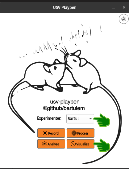
In order to run any of the functions detailed below, select an experimenter name from the dropdown menu and click the Visualize button on the GUI main display:

Clicking the Visualize button will open a new window with all the offered functionalities (see below):

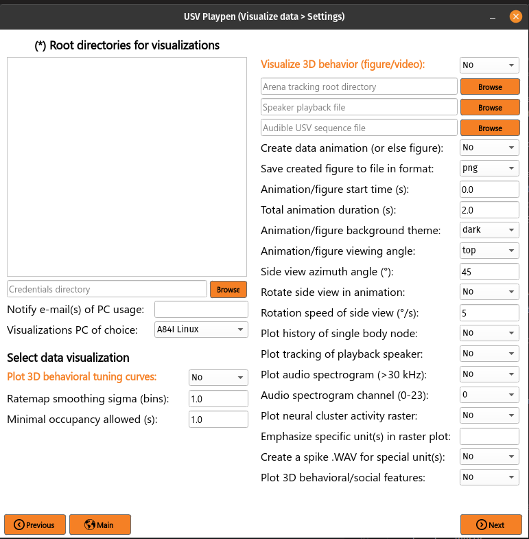
All the main functions are outlined in orange, and black fields are function-specific options tunable by the user in the GUI. It is important to note that these are not necessarily all the options the user can set, and the full list of options can be found under each function in the /usv-playpen/_parameter_settings/visualizations_settings.json file. Each time the user clicks the Next button in the window above, visualizations_settings.json is modified to the newest input configuration.

The Root directories field enables you to list the directories containing the data you want to visualize. Each root directory should be in its own row; for example, three sessions should be listed as follows:

/mnt/falkner/Bartul/Data/20250430_145017
/mnt/falkner/Bartul/Data/20250430_165730
/mnt/falkner/Bartul/Data/20250430_182145

Plot neuronal tuning figures

Once the Compute neuronal tuning curves function from the Analyze section has completed, you have the ability to plot its results. Output is one combined multi-page document per cluster: a behavioral page per temporal offset and per plot-feature group (individual.<mouse> and social) followed by two vocal pages — the first (bout raster + pooled pre-USV (ultrasonic vocalization) usv_peth on top, usv_property_tuning continuous-property grid below) and the second (usv_category_tuning watersheds (the watershed segmentation algorithm) + usv_category_peth per-category PETH (peri-event time histogram) grid). 1D ratemaps are drawn as a line spanning the plot, colored by the per-mouse palette (or the social color for social features). The 99% CI (confidence interval) of the shuffled distribution is shown as a shaded band around the line.

To obtain this visualization, list the root directories of interest, select Plot neuronal tuning figures in the GUI and click Next and then Visualize:

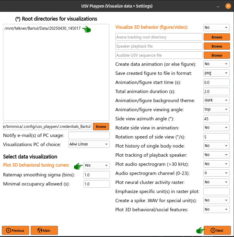
Running this function results in the population of the tuning_curves subdirectory with one combined output per cluster (PDF by default; configurable in the GUI / settings):

├── 20250430_145017
│   ├── audio
│   │   ...
│   ├── ephys
│   │   ├── tuning_curves
│   │   │   ├── imec0_cl0000_ch361_good_neuronal_tuning.pdf
│   │   │   ...
│   ├── sync
│   │   ...
│   └── video
│       ...

For non-PDF formats, each page is written to a separate file with a _p{N}_{label} suffix (e.g. ..._p1_behavioral_beh_offset=0s_individual.<mouse>.png, ..._p3_vocal_a_male.png). PDF emits a single multi-page file.

The rendering-side knobs live in the project-wide figures block of /usv-playpen/_parameter_settings/visualizations_settings.json (compute-side knobs such as smoothing_sd and behavioral_min_occupancy_seconds live in analyses_settings.json under calculate_neuronal_tuning_curves — see the Analyze page):

• save_directory : default output directory for figures that aren’t written next to their source data (e.g. cross-session anatomy plots). Per-figure code may override this with an explicit out_dir argument; per-cluster ratemaps and other session-bound figures always stay next to the data.

• fig_format : default output file format. For the per-cluster ratemap PDFs, pdf produces a single multi-page document; png / jpg / svg write one file per page.

• dpi : default raster resolution applied to every fig.savefig callsite that goes through visualizations.figure_io.save_figure.

• timestamp_in_name : when true, _YYYYMMDD_HHMMSS is appended to figure stems by default. Session-bound figures opt out of this with timestamp_in_name=false since their filenames already embed a session id or unit id.

• cmap : default matplotlib colormap used by every heatmap / ratemap callsite (one of viridis, cividis, plasma, inferno, magma); the make_behavioral_videos spectrogram subplot and the qlvm_torus_traversal_video spectrogram tiles also read it.

• seed : random seed for figure-side stochastic operations, for reproducibility.

"figures": {
    "save_directory": "/mnt/falkner/Bartul/figures",
    "fig_format": "png",
    "dpi": 300,
    "timestamp_in_name": true,
    "cmap": "inferno",
    "seed": 0
}

Colour palettes

Top-level *_colors blocks in visualizations_settings.json hold the semantic (data-meaning) colours shared across figures; every entry is a hex string, so a whole figure family can be recoloured in one place. Sex / emitter colours are lists (index 0 primary, 1 secondary) while the grouped palettes are named maps.

• male_colors / female_colors / unassigned_colors : per-emitter USV colours (male / female / no-emitter-assigned), used by the USV-timeline, spectrogram-overlay, embedding-scatter and modeling figures.

• social_colors : the single colour for social / dyadic features (e.g. the social-feature ratemaps and the timescale-audit “social” trace).

• brain_area_colors : per-brain-region palette (a seven-bucket map: PAG / MRN / VTA / SC / CENT / MB / other) shared by the behavioral-video overlays and the anatomy / tuning figures.

• cell_type_colors : the mono-grey triad for the per-mouse cell-type stacked bars in the anatomy figures.

• coactivity_colors : the group_a / group_b / null / threshold colours for the neuronal-coactivity figures (also the defaults the coactivity notebook may override inline).

• component_colors : the per-mixture-component colour cycle for the inter-USV-interval mixture-model figures (paired in code with distinct line styles).

• corner_colors : the arena-corner marker colours (North / West / South / East) for the behavioral-video arena overlay.

"male_colors": ["#9AC0CD", "#8CA252"],
"female_colors": ["#FF6347", "#B851B4"],
"social_colors": ["#5A6470"],
"unassigned_colors": ["#C0C0C0"],
"brain_area_colors": {"PAG": "#677470", "MRN": "#939884", "VTA": "#F5D27A",
                      "SC": "#9FB7D8", "CENT": "#D88080", "MB": "#9BBE85", "other": "#B8B8B8"},
"cell_type_colors": ["#1A1A1A", "#7A7A7A", "#CFCFCF"],
"coactivity_colors": {"group_a": "#DC143C", "group_b": "#1E90FF", "null": "#808080", "threshold": "#000000"},
"component_colors": ["#1f77b4", "#ff7f0e", "#2ca02c", "#d62728",
                     "#9467bd", "#8c564b", "#e377c2", "#7f7f7f"],
"corner_colors": {"North": "#FF0000", "West": "#FFFF00", "South": "#008000", "East": "#0000FF"}

Visualize 3D behavior (figure/video)

Once 3D tracked data is available, you can visualize animal social behavior, either in figure or video. This GUI segment allows for a wide array of options in creating such visualizations. For example, you can choose whether you want to view the interaction from above or the side, and you can also choose to rotate the view as the behavior unfolds.

To obtain this visualization, you need to list the root directories of interest (it is best to stick with one), select the Visualize 3D behavior (figure/video) option in the GUI, insert the arena directory for that session, pick all desired figure features, click Next and then Visualize. It is important to point out that there are many more features available in the visualizations_settings.json file than are available in the GUI, and these options are explained in detail several sections below:

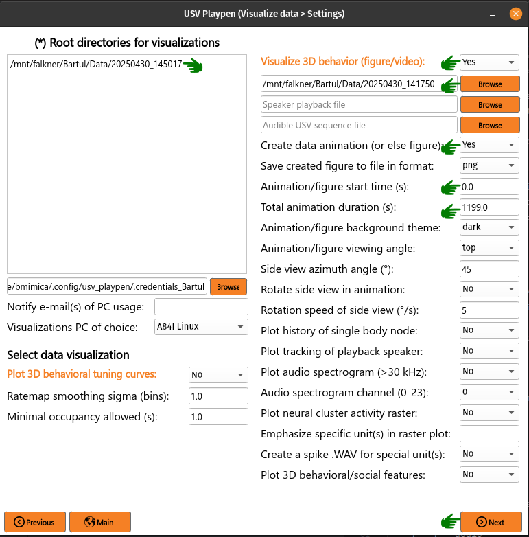
Running this function results in the creation of the data_animation_examples subdirectory (if it has not been created already), and the figure/video will be saved inside:

├── 20250430_145017
│   ├── audio
│   │   ...
│   ├── data_animation_examples
│   │   ├── 20250430_145017_3D_30045fr_dark_topview_17features_spectrogram_ch0_Bartul_20260701_133612.png
│   │   ├── 20250430_145017_3D_30045-30795fr_dark_topview_17features_spectrogram_ch0_Bartul.mp4
│   │   ...
│   ├── ephys
│   │   ...
│   ├── sync
│   │   ...
│   └── video
│       ...

The /usv-playpen/_parameter_settings/visualizations_settings.json file contains a section only partially modifiable in the GUI, but it can entirely be modified manually in the visualizations_settings.json file:

• arena_directory : path to the directory with the 3D tracked arena data

• speaker_audio_file : path to the audio file containing the playback speaker sound

• pitch_shifted_audio_bool : if “Yes”, automatically frequency-shift the session USVs over the chosen [video_start_time, video_start_time + video_duration] window into the human-audible range and mux the result onto the video (replaces the former manual sequence_audio_file path)

• pitch_shifted_audio_specs : pitch-shift recipe used when pitch_shifted_audio_bool is “Yes” (fs_audio_dir, fs_device_id, fs_channel_id, fs_wav_sampling_rate, fs_octave_shift, fs_volume_adjustment, fs_compand_transfer, fs_noise_reduction_std_threshold, fs_sinc_upper_cutoff_hz)

• animate_bool : boolean value indicating whether to animate the figure or not (“No” creates figure)

• video_start_time : start time of the figure/video in seconds

• video_duration : duration of the video in seconds

• plot_theme : “dark” or “light” plot background

• save_fig : if True, the figure will be saved in the data_animation_examples subdirectory

• view_angle : “top” or “side” view of social behavior in the playpen arena

• side_azimuth_start : azimuth angle of the side view (in deg)

• rotate_side_view_bool : rotate the side view or not (NB: angles wrap around)

• rotation_speed : rotation speed of the side view (in deg/s)

• history_bool : plot the location history of one body node

• speaker_bool : plot the playback speaker

• spectrogram_bool : plot the spectrogram of the audio segment

• spectrogram_ch : channel of the audio segment to plot

• raster_plot_bool : plot the live spiking raster of the neural data

• raster_selection_criteria : criteria for selecting the neurons to plot in the raster

• raster_selection_criteria (brain_areas) : list of brain areas to include in the raster plot

• raster_selection_criteria (other) : list of other criteria to include in the raster plot (e.g., “good” for unit type)

• raster_special_units : unit(s) to highlight in the raster plot (e.g., “imec0_cl0000_ch361”)

• spike_sound_bool : make spike sound each time the highlighted unit spikes

• beh_features_bool : plot the behavioral features dynamics subplot

• beh_features_to_plot : list of behavioral features in the subplot

• special_beh_features : list of highlighted behavioral features in the subplot

Parameters controlling the figure output format and video encoding (general_figure_specs):

• fig_format : output image format for still frames (e.g. “png”).

• animation_codec : FFMPEG video codec for the rendered animation (e.g. “h264_nvenc”).

• animation_codec_preset_flag : codec preset / speed-quality flag (e.g. “p5”).

• animation_codec_tune_flag : codec tuning flag (e.g. “hq”).

• animation_writer : matplotlib animation writer (e.g. “ffmpeg”).

• animation_format : output video container format (e.g. “mp4”).

Parameters specific to the arena figure include:

• arena_node_connections_bool : plots connections between corner and nearest microphones

• arena_axes_lw : line width of the arena axes

• arena_mics_lw : line width of the microphones

• arena_mics_opacity : opacity of the microphones

• plot_corners_bool : plot different color spheres in corners of the arena

• corner_size : size of the corner spheres

• corner_opacity : opacity of the corner spheres

• plot_mesh_walls_bool : plot the mesh walls of the arena

• mesh_opacity : opacity of the mesh walls

• active_mic_bool : plots the active microphone (whose spectrogram is shown)

• inactive_mic_bool : plots the inactive microphones (whose spectrograms are not shown)

• inactive_mic_color : color of the inactive microphones

• text_fontsize : font size of the text in the arena figure

• speaker_opacity : opacity of the playback speaker

Parameters specific to the mouse figure include:

• node_bool : plot mouse body nodes as spheres

• node_size : size of the body node spheres

• node_opacity : opacity of the body node spheres

• node_lw : line width of the body node spheres

• node_connection_lw : plots connections between body nodes

• body_opacity : opacity of the body polygons connected with nodes

• history_point : plot history of particular body point

• history_span_sec : time span of the history in seconds (will fail if history is set to start before tracking!)

• history_ls : line style of the history plot (e.g., “-”, “–”, “-.”, “:”)

• history_lw : line width of the history plot

Parameters specific to subplots include:

• beh_features_window_size : time window of the behavioral features subplot (in s, will fail if is set beyond tracking boundaries!)

• raster_window_size : time window of the raster subplot (in s, will fail if is set beyond tracking boundaries!)

• raster_lw : horizontal line width of spikes in the raster plot

• raster_ll : vertical line length of spikes in the raster plot

• spectrogram_cbar_bool : plot spectrogram colorbar

• spectrogram_plot_window_size : time window of the spectrogram subplot (in s, will fail if is set beyond tracking boundaries!)

• spectrogram_power_limit : lower and upper limits of the spectrogram colorbar (in dB)

• spectrogram_frequency_limit : lower and upper limits of the spectrogram frequency axis (in Hz)

• spectrogram_yticks : y-axis ticks of the spectrogram (in Hz)

• spectrogram_stft_nfft : window size for the spectrogram calculation

• plot_usv_segments_bool : plot the Deep Audio Segmenter (DAS)-detected USV segments in the spectrogram

• usv_segments_ypos : y-axis position of the USV segments in the spectrogram (in Hz)

• usv_segments_lw : line width of the USV segments in the spectrogram

"make_behavioral_videos": {
    "arena_directory": "",
    "speaker_audio_file": "",
    "pitch_shifted_audio_bool": false,
    "pitch_shifted_audio_specs": {
        "fs_audio_dir": "hpss_filtered",
        "fs_device_id": "m",
        "fs_channel_id": 1,
        "fs_wav_sampling_rate": 250,
        "fs_octave_shift": -3,
        "fs_volume_adjustment": true,
        "fs_compand_transfer": "0.3,1 6:-70,-60,-20 -5 -90 0.2",
        "fs_noise_reduction_std_threshold": 3,
        "fs_sinc_upper_cutoff_hz": 25000
    },
    "animate_bool": false,
    "video_start_time": 37.0,
    "video_duration": 10.0,
    "plot_theme": "dark",
    "save_fig": true,
    "view_angle": "top",
    "side_azimuth_start": 45,
    "rotate_side_view_bool": false,
    "rotation_speed": 20,
    "history_bool": false,
    "speaker_bool": false,
    "spectrogram_bool": false,
    "spectrogram_ch": 0,
    "raster_plot_bool": false,
    "raster_selection_criteria": {
      "brain_areas": [],
      "other": [
        "good"
      ]
    },
    "raster_special_units": [
      ""
    ],
    "spike_sound_bool": false,
    "beh_features_bool": false,
    "beh_features_to_plot": [],
    "special_beh_features": [],
    "general_figure_specs": {
      "fig_format": "png",
      "animation_codec": "h264_nvenc",
      "animation_codec_preset_flag": "p5",
      "animation_codec_tune_flag": "hq",
      "animation_writer": "ffmpeg",
      "animation_format": "mp4"
    },
    "arena_figure_specs": {
      "arena_node_connections_bool": false,
      "arena_axes_lw": 1.0,
      "arena_mics_lw": 0.75,
      "arena_mics_opacity": 0.25,
      "plot_corners_bool": false,
      "corner_size": 1.0,
      "corner_opacity": 1.0,
      "plot_mesh_walls_bool": true,
      "mesh_opacity": 0.1,
      "active_mic_bool": false,
      "inactive_mic_bool": true,
      "inactive_mic_color": "#898989",
      "text_fontsize": 10,
      "speaker_opacity": 1.0
    },
    "mouse_figure_specs": {
      "node_bool": true,
      "node_size": 3.5,
      "node_opacity": 1.0,
      "node_lw": 0.5,
      "node_connection_lw": 1.0,
      "body_opacity": 0.85,
      "history_point": "Head",
      "history_span_sec": 5,
      "history_ls": "-",
      "history_lw": 0.75
    },
    "subplot_specs": {
      "beh_features_window_size": 10,
      "raster_window_size": 1,
      "raster_lw": 0.3,
      "raster_ll": 10.9,
      "spectrogram_cbar_bool": true,
      "spectrogram_plot_window_size": 1,
      "spectrogram_power_limit": [
        -60,
        0
      ],
      "spectrogram_frequency_limit": [
        30000,
        125000
      ],
      "spectrogram_yticks": [
        50000,
        100000
      ],
      "spectrogram_stft_nfft": 512,
      "plot_usv_segments_bool": true,
      "usv_segments_ypos": 120000,
      "usv_segments_lw": 1.25
    }
}

Render the QLVM torus-traversal

The usv_playpen.visualizations.qlvm_torus_traversal_video module renders a two-panel toroidal (doughnut-shaped) “torus walkthrough” animation (the in-house, torch-free port of qmc_deep_gen’s inference_latents_video.py). The left panel is the QLVM (the in-house quasi-Monte Carlo latent variable model) latent map — the density heatmap with watershed cluster contours (no axes/ticks) and a recency-coloured trajectory trail (cyan at the current position, fading to white going back, built with create_colormap); the right panel is a phase-specific spectrogram board. All spectrograms have their SAM2 (Segment Anything Model 2) mask applied (apply_mask) and the call centred in its window with equal padding on both sides (so duration is preserved, not stretched). It runs in three parts, each introduced by a title card:

• Part 1 — Cluster peaks: one phase per cluster, the right panel showing that cluster’s peak spectrogram surrounded by its m nearest USVs in concentric rings; on the left the active cluster is outlined in a thick pulsating cyan contour with a cyan dot at its centre.

• Part 2 — Peak-to-peak walks: shortest-torus-path walks between random cluster peaks; the right 5×15 grid fills row-major with the nearest USV at each visited position (the current tile bordered in cyan).

• Part 3 — Boundary crossings: curved walks that wrap the torus edges/corners; the right grid’s columns are trajectory positions and rows are nearest neighbours (the current trajectory tile bordered in cyan).

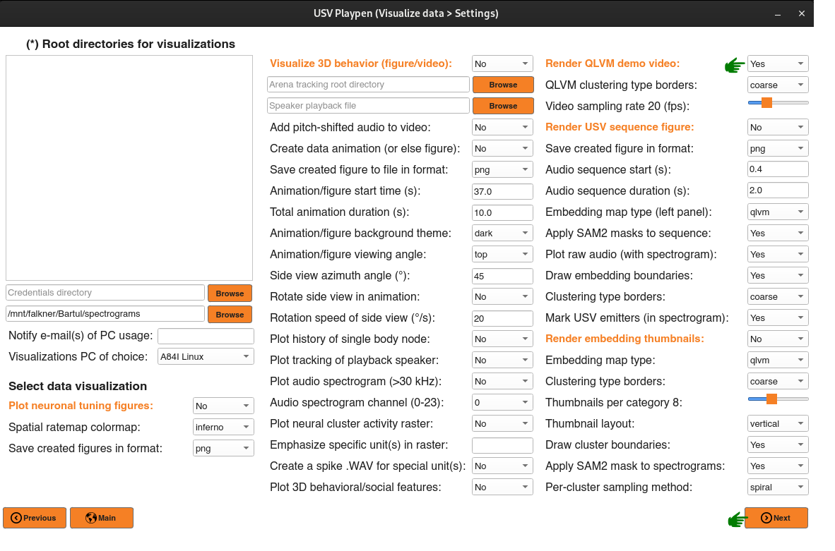
It is cohort-level — it reads one model’s analysis arrays + the consolidated store, not a session directory — and is exposed both as the qlvm-torus-traversal-video CLI and in the GUI Visualize window (third column): “Render QLVM demo video” (Yes/No), a QLVM clustering type borders selector (coarse = 7 clusters / fine = 12), and a Video sampling rate (fps) slider. A single Spectrograms directory Browse field lives in the left column under Credentials directory (the shared shared_resources.spectrograms_dir base, under which the QLVM arrays and the consolidated store are resolved by convention).

To render it, list a root directory, set the Spectrograms directory, select Render QLVM demo video, choose the clustering and Video sampling rate (fps), click Next and then Visualize:

Inputs — both resolved by convention via configure_path from the single shared_resources.spectrograms_dir base (shared with the USV sequence figure and the stitched spectrogram):

• <spectrograms_dir>/qlvm/arrays_{coarse,fine}.npz — the QLVM analysis arrays, used ONLY for the heatmap background, ws_labels_periodic cluster contours, and centers (the cluster peaks / path waypoints); the QLVM clustering type borders selector picks which one.

• <spectrograms_dir>/spectrograms_*.h5 (newest match) — the consolidated per-session spectrogram/SAM2 store. It supplies BOTH the per-USV latent coords (per-session spectrogram/<key>/qlvm_dim) for the nearest-neighbour lookup AND the spectrograms (spectrogram/<key>/spectrograms) shown on the right. No latents pickle is read at render time, and coverage spans all sessions in the store.

One-time prerequisite — the consolidated H5 does not ship with latent coordinates, so it must be enriched once with a small per-session spectrogram/<key>/qlvm_dim (n, 2) dataset (a few MB, non-destructive — existing spectrograms/masks are untouched), populated from the latents provenance pickle. This is a one-off data migration (a throwaway script, not a repo command). If the video is run before the store has qlvm_dim it raises a clear error.

Because it is cohort-level, the output is not written next to a session; the .mp4 lands in the project-wide figures.save_directory with a render-timestamped name (qlvm_torus_traversal_<YYYYMMDD_HHMMSS>.mp4) unless an explicit --output-path is given:

├── ...  (the figures.save_directory cohort output folder)
│   ├── qlvm_torus_traversal_20250430_145017.mp4
│   ...

The render parameters live in the qlvm_torus_traversal_video block of /usv-playpen/_parameter_settings/visualizations_settings.json:

• clustering : which cluster set to traverse — coarse (7 clusters) or fine (12); set by the GUI QLVM clustering type borders selector.

• fps : output frame rate.

• dpi : raster resolution of each rendered frame.

• m : number of nearest-neighbour USVs shown in the concentric rings around each cluster peak (Part 1).

• cluster_hold_frames : frames each cluster peak is held on screen (Part 1).

• peak_traverse_frames : frames spent on each peak-to-peak walk (Part 2).

• boundary_traverse_frames : frames spent on each boundary-crossing walk (Part 3).

• title_card_frames : frames each of the three title cards is shown.

• samples_per_trace : number of positions revealed along each peak-to-peak walk (one nearest neighbour each).

• peak_jitter_sigma : random jitter (torus units) applied to the peak-walk trajectory so repeated paths do not overlap.

• boundary_curve_amplitude : curvature amplitude of the Part-3 boundary walks.

• boundary_positions_per_walk : number of positions revealed along each boundary walk.

• boundary_neighbors : nearest neighbours shown per boundary position (the Part-3 grid rows).

• seed : RNG (random-number-generator) seed for the walks / jitter (reproducible renders).

• peaks_only : when true, render Part 1 (cluster peaks) only.

• spec_cache_size : number of spectrograms held in the in-memory LRU cache during rendering.

• apply_mask : apply the SAM2 mask to each spectrogram.

• accent_color : hex highlight color for the trail / head marker / cluster outline + dot / current-tile borders.

"qlvm_torus_traversal_video": {
    "clustering": "coarse",
    "fps": 20,
    "dpi": 100,
    "m": 36,
    "cluster_hold_frames": 60,
    "peak_traverse_frames": 200,
    "boundary_traverse_frames": 200,
    "title_card_frames": 45,
    "samples_per_trace": 75,
    "peak_jitter_sigma": 0.015,
    "boundary_curve_amplitude": 0.18,
    "boundary_positions_per_walk": 15,
    "boundary_neighbors": 5,
    "seed": 0,
    "peaks_only": false,
    "spec_cache_size": 2048,
    "apply_mask": true,
    "accent_color": "#00FFFF"
}

Render a USV sequence figure

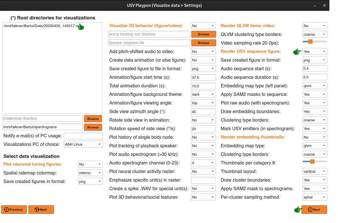
USVSpectrogramPlotter.plot_sequence (the 'sequence' mode of make_usv_spectrograms) renders a per-session, static two-panel figure of the USVs in a chosen [start, start + duration] window (seconds). It is wired into the GUI Visualize window (third column) under “Render USV sequence figure” and dispatched per session in visualize_data.py via make_usv_spectrograms_bool (enabling the GUI toggle sets make_usv_spectrograms.mode = 'sequence').

To render it, list a session root, select Render USV sequence figure, set the audio-sequence window and options, click Next and then Visualize:

• Left — a precomputed cohort embedding landscape (embedding = qlvm or vae), drawn with no ticks/ticklabels. The window’s USVs are colored by emitter (male_colors[0] / female_colors[0] / unassigned_colors[0]), sized by call duration, numbered 1..n in time order, and joined by a connecting line whose color runs white → male color along the bout and whose per-segment width tracks the inter-USV silent gap (start of the next minus stop of the previous; on the QLVM torus the line takes the short wrap-around route across an edge when that is closer — VAE (variational autoencoder) is a plain plane, no wrapping). Both embeddings draw a gray_r density heatmap and, when draw_boundaries is on, overlay black category boundaries selected by boundary_clustering (coarse / fine). Both maps are resolved by convention from the shared shared_resources.spectrograms_dir: QLVM from <dir>/qlvm/arrays_{coarse,fine}.npz (the watershed arrays, on the unit torus); VAE from <dir>/vae/vae_density_{coarse,fine}.npz (a cohort density precomputed over the umap (Uniform Manifold Approximation and Projection) coordinate extent), where coarse = vae_supercategory and fine = vae_category regions. The VAE files are built once with build_vae_density_npz (CLI build-vae-density), which pools the cohort via build_pooled_embeddings_df, histograms a density, and rasterizes a nearest-neighbour category field. VAE still requires the session’s usv_summary to carry vae_umap1/vae_umap2 (else a clear error is raised); when the resolved npz is absent (e.g. the VAE density was never precomputed) the panel falls back to a bare (tick-free) scatter.

• Right — ONE continuous spectrogram over the same window: the per-USV averaged spectrograms are SAM2-masked (when apply_mask) and stitched at their true times onto a black background, so only the calls are lit and the gaps are black; an optional raw-audio trace can sit on top (plot_raw_audio), taken from the channel that is loudest across the window’s USVs (the most-frequent per-USV peak_amp_ch; raw waveforms are NOT averaged across mics — the per-mic phase delays would interfere destructively). Each USV can also be marked with a horizontal emitter-colored bar along the top of the spectrogram (mark_usv_segments). The left-panel numbers match the time order of the calls along the right time axis.

The GUI section leads with a Save created figure in format selector (writes make_usv_spectrograms.fig_format); Draw embedding boundaries applies to both embeddings, and Clustering type borders is greyed out unless boundaries are drawn.

The QLVM arrays, the VAE density arrays, and the consolidated store are all resolved by convention from the single shared_resources.spectrograms_dir base (qlvm/arrays_{coarse,fine}.npz, vae/vae_density_{coarse,fine}.npz, the newest spectrograms_*.h5). Being per-session, the figure is written to save_dir — or, when that is empty, to the data_animation_examples subdirectory of the session (the same per-session output folder the behavioral videos use) — and, when auto_open_figure is on AND running in a GUI context, opened in the OS default viewer (headless / batch runs never spawn a viewer; the plotter closes each figure after saving so a per-session run does not accumulate open figures):

├── 20250430_145017
│   ├── audio
│   │   ...
│   ├── data_animation_examples
│   │   ├── usv_spectrogram_..._sequence_qlvm_from_0.4s_to_2.4s_20250430_145017.png
│   │   ...
│   ├── ephys
│   │   ...
│   ├── sync
│   │   ...
│   └── video
│       ...

Settings live in the make_usv_spectrograms block of /usv-playpen/_parameter_settings/visualizations_settings.json — the shared top-level keys:

• save_dir : output directory; empty routes the figure to the session’s data_animation_examples folder.

• save_fig : whether to write the figure to disk.

• fig_format : output file format (png / pdf / svg / jpg).

• fig_dpi : raster resolution.

• fig_size : figure size in inches ([width, height]).

• transparent_fig_bg : save the figure on a transparent background.

• mode : the figure type the make_usv_spectrograms class renders. For this figure it is pinned to sequence — the GUI toggle overwrites it, so it is not a choice here. It becomes a free selection only when the plotter is driven from usv_general_analyses.ipynb (see Notebooks), where the other values render different figures (single / all = raw per-channel spectrograms; stitched = the averaged session-timeline spectrogram).

• channel_of_interest : microphone channel for the single mode (unused by sequence, which auto-selects the loudest channel over the window).

• plot_raw_audio : overlay the raw-audio amplitude trace on the stitched spectrogram.

• usv_amplitude_color : hex color of that raw-audio amplitude trace.

• time_window : [start, end] seconds of the window (the GUI presents it as a start + duration pair and writes it back).

• freq_limits : [low, high] kHz frequency axis of the spectrogram.

• nfft : FFT window size for the spectrogram.

• plot_cbar : whether to draw the colorbar.

• cbar_limits : [vmin, vmax] colorbar (power) limits in dB.

• apply_mask : apply the SAM2 mask to each per-USV spectrogram before stitching.

• auto_open_figure : open the saved figure in the OS viewer when running in a GUI context.

plus the sequence sub-dict:

• embedding : left-panel landscape — qlvm (torus) or vae (umap plane).

• draw_boundaries : overlay category boundaries on the left panel.

• boundary_clustering : which boundary set — coarse / fine.

• annotate_right : annotate the stitched (right) spectrogram.

• mark_usv_segments : draw an emitter-colored bar along the top of the spectrogram for each USV.

"make_usv_spectrograms": {
    "save_dir": "",
    "save_fig": true,
    "fig_format": "png",
    "fig_dpi": 300,
    "fig_size": [6, 2],
    "transparent_fig_bg": false,
    "mode": "sequence",
    "channel_of_interest": 11,
    "plot_raw_audio": true,
    "time_window": [0.4, 2.4],
    "freq_limits": [40, 95],
    "usv_amplitude_color": "#808080",
    "nfft": 512,
    "plot_cbar": true,
    "cbar_limits": [-70, 0],
    "apply_mask": true,
    "auto_open_figure": true,
    "sequence": {
        "embedding": "qlvm",
        "draw_boundaries": true,
        "boundary_clustering": "coarse",
        "annotate_right": false,
        "mark_usv_segments": true
    }
}

Render embedding thumbnails

The usv_playpen.visualizations.make_usv_spectrograms module’s remaining cohort-level helper, plot_embedding_with_category_thumbnails, is GUI-exposed (its pooled summary helpers — plot_usv_property_histograms, plot_session_type_usv_counts, plot_session_usv_timeline — are notebook-driven; see Notebooks):

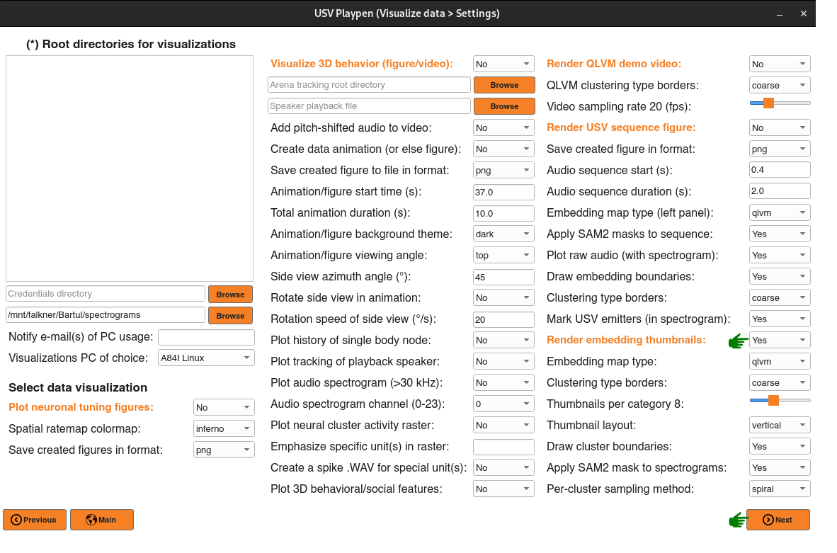
• plot_embedding_with_category_thumbnails — a two-panel figure pairing an embedding scatter (VAE umap or QLVM torus) — colored by call category and overlaid with kNN (k-nearest-neighbors) cluster boundaries — against a per-category grid of spectrogram thumbnails sampled from the consolidated SAM2 + spectrogram store. Unlike the helpers above it is cohort-level and exposed in the GUI: enabling Render embedding thumbnails in the Visualize window (third column, with map type, clustering type borders (coarse / fine), thumbnails per category, thumbnail layout, draw cluster boundaries, apply SAM2 mask and per-cluster sampling selectors) pools every cohort session list under shared_resources.input_files_directory and resolves the store from shared_resources.spectrograms_dir, then runs ONCE (the same run-once dispatch as the QLVM torus video, via render_embedding_thumbnails_for_cohort). Its layout / sampling knobs all live in the embedding_thumbnails settings block (documented below); the figure DPI and the sampling seed are taken from the general figures block (dpi / seed); the QLVM cluster centers (for cluster-ID labels / spiral centers) are auto-resolved from the newest qlvm_clusters_*.h5 under spectrograms_dir (QLVM map only); and the cohort scatter is read from the precomputed pooled-embeddings cache <spectrograms_dir>/embeddings/pooled_embeddings.parquet (one parquet holding both embeddings’ coordinates and the coarse + fine labels) — built once on a fast mount via build_pooled_embeddings_df so the figure does not re-read every session’s usv_summary.csv.

To render it, select Render embedding thumbnails in the Visualize window, choose the map / clustering / layout options, click Next and then Visualize:

Being cohort-level, the figure is written to the project-wide figures.save_directory with a name built from the map and label column (plus a _YYYYMMDD_HHMMSS stamp when figures.timestamp_in_name is set):

├── ...  (the figures.save_directory cohort output folder)
│   ├── embedding_thumbnails_qlvm_supercategory_20250430_145017.png
│   ...

The layout / sampling knobs live in the embedding_thumbnails block of /usv-playpen/_parameter_settings/visualizations_settings.json (the figure DPI and the sampling seed come from the general figures block). Core keys:

• map_type : embedding to plot — qlvm (torus) or vae (umap).

• category_col_suffix : the label column that colors / groups the scatter and thumbnail rows — category or supercategory.

• n_samples_per_category : number of thumbnail spectrograms sampled per category.

• tile_orientation : thumbnail grid orientation — vertical / horizontal.

• apply_mask : apply the SAM2 mask to each thumbnail spectrogram.

• mask_excluded_categories : categories to omit from the thumbnail grid.

• category_colors : optional explicit per-category color map (null = auto).

• scatter_max_points : downsampling cap for the embedding scatter.

Sampling / boundaries:

• sampling_method : how thumbnails are drawn per category (e.g. spiral).

• draw_cluster_boundaries : overlay kNN cluster boundaries on the scatter.

• knn_boundary_neighbors : k for the kNN boundary field.

• knn_boundary_resolution : grid resolution of the boundary field.

• knn_boundary_density_min_count : minimum density (fraction) below which no boundary is drawn.

• knn_boundary_density_smoothing_sigma : Gaussian smoothing sigma of the boundary density.

Spiral overlay:

• draw_spiral_overlay : draw the sampling-spiral overlay on the scatter.

• spiral_show_only_for : restrict the overlay to one category (null = all).

• spiral_color : hex color of the spiral.

• spiral_linewidth : spiral line width.

• spiral_radius_scale / spiral_radius_abs : spiral radius (relative / absolute).

• spiral_n_turns : number of spiral turns.

• spiral_random_phase : randomize the spiral’s starting angle.

Annotations / layout:

• annotate_picks_on_scatter : number each sampled pick on the scatter.

• pick_number_fontsize : font size of those pick numbers.

• annotate_cluster_ids : label each cluster with its id.

• cluster_id_fontsize : font size of the cluster-id labels.

• thumbnail_hspace / thumbnail_wspace : vertical / horizontal spacing between thumbnails.

• unstretched_specs : keep thumbnails at their native aspect (no stretch).

• fig_size : figure size in inches ([width, height]).

"embedding_thumbnails": {
    "map_type": "qlvm",
    "category_col_suffix": "supercategory",
    "n_samples_per_category": 8,
    "tile_orientation": "vertical",
    "apply_mask": true,
    "mask_excluded_categories": [],
    "category_colors": null,
    "sampling_method": "spiral",
    "draw_cluster_boundaries": true,
    "knn_boundary_neighbors": 15,
    "knn_boundary_resolution": 200,
    "knn_boundary_density_min_count": 0.05,
    "knn_boundary_density_smoothing_sigma": 3.0,
    "draw_spiral_overlay": false,
    "spiral_show_only_for": null,
    "spiral_color": "#000000",
    "spiral_linewidth": 1.0,
    "spiral_radius_scale": 0.1,
    "spiral_radius_abs": 0.1,
    "spiral_n_turns": 3,
    "spiral_random_phase": true,
    "annotate_picks_on_scatter": false,
    "pick_number_fontsize": 9,
    "annotate_cluster_ids": true,
    "cluster_id_fontsize": 20,
    "thumbnail_hspace": 0.03,
    "thumbnail_wspace": 0.04,
    "unstretched_specs": true,
    "scatter_max_points": 200000,
    "fig_size": [16, 12]
}