Process
This page explains how to use the data processing functionalities in the usv-playpen GUI.
In order to run any of the functions detailed below, select an experimenter name from the dropdown menu and click the Process button on the GUI main display:
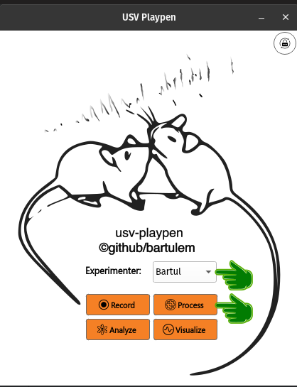
Clicking the Process button will open a new window with all the processing functionalities (see below):
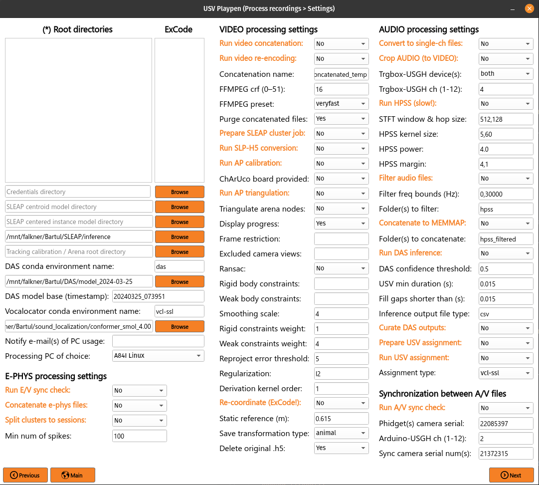
All the main functions are outlined in orange, and black fields are function-specific options tunable by the user in the GUI. It is important to note that these are not necessarily all the options the user can set, and the full list of options can be found under each function in the /usv-playpen/_parameter_settings/processing_settings.json file. Each time the user clicks the Next button in the window above, processing_settings.json is modified to the newest input configuration.
Note
The shipped *_settings.json files store a literal default experimenter
(by default Bartul). Experimenter-scoped paths are re-keyed to the active
experimenter automatically: in the GUI from the front-page experimenter
selection, and for headless / CLI / cluster runs from the host
behavioral_experiments_settings.toml experimenter key. You therefore
set your experimenter once instead of editing every path; the example paths
below show that shipped default.
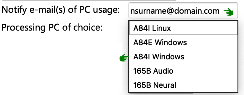
It is relevant to note here, that just like in the Record section, you have the capability to Notify e-mail(s) of PC usage. This is useful if you are running a long processing job and want to be notified when it is finished. The e-mails about start and end of jobs will be sent to the addresses listed in the Notify e-mail(s) of PC usage field (no space after comma for multiple e-mails), and it requires you to choose what particular PC you are using for this job. Since the e-mails are sent from a Google account, the first e-mail you receive may end up in the Spam folder, so make sure to check that:
The Root directories field enables you to list the directories containing the data you want to process. Each root directory should be in its own row; for example, three sessions should be listed as follows:
/mnt/falkner/Bartul/Data/20250430_145017
/mnt/falkner/Bartul/Data/20250430_165730
/mnt/falkner/Bartul/Data/20250430_182145
Certain processing functions take all root sessions together when operating on data, and others process each session separately. Additionally, in both of these categories, there is a specific order in executing individual functions.
For combined processing, the order of processing steps is as follows:
Concatenate e-phys files
Split clusters to sessions
Prepare SLEAP cluster job
Build QLVM training set (CLI only)
Train QLVM (CLI only)
Export YOLO dataset (CLI only)
Train (spectrogram) masks (CLI only)
The last four run only when (re)training the spectrogram-pipeline models: they aggregate a cohort of sessions and produce the QLVM (the in-house quasi-Monte Carlo latent variable model) decoder and You Only Look Once (YOLO) object detector weights that the per-session Infer QLVM latents / Generate (spectrogram) masks steps reload (see the Render spectrograms and latents section below).
On the other hand, for processing sessions separately, the order of processing steps is as follows:
Run video concatenation
Run video re-encoding
Convert to single-ch files
Crop AUDIO (to VIDEO)
Run A/V sync check
Run E/V sync check
Run HPSS
Filter audio files
Concatenate to MEMMAP
Run SLP-H5 conversion
Run AP calibration
Run AP triangulation
Re-coordinate
Run DAS inference
Curate DAS outputs
Prepare USV assignment
Run USV assignment
Generate spectrograms
Generate (spectrogram) masks
Compute USV features
Infer QLVM latents
If you recorded a session with audio, e-phys and video data (imaginary example: 20250430_145017) and a calibration session (20250430_142022), the directory and file structure should look as follows:
/mnt/falkner/Bartul/Data/:
├── 20250430_145017
│   ├── 20250430_145017_metadata.yaml
│   ├── audio
│   │   ├── original (empty)
│   │   ├── original_mc
│   │       ├── m_250430145009.wav
│   │           ...
│   │   ├── audio_triggerbox_sync_info.json
│   ├── ephys
│   │   ├── imec0
│   │   │   ├── 20250430_145017.imec0.ap.bin
│   │   │   ├── 20250430_145017.imec0.ap.meta
│   │   ├── imec1
│   │       ├── 20250430_145017.imec1.ap.bin
│   │       ├── 20250430_145017.imec1.ap.meta
│   ├── sync
│   │   ├── CoolTerm Capture (coolterm_config.stc) 2024-04-30-14-50-14-236.txt
│   │   ├── 20250430_rec4_g0_t0.nidq.bin
│   │   ├── 20250430_rec4_g0_t0.nidq.meta
│   │
│   └── video
│       ├── 20250430_145027.21241563
│           ├── 000000.mp4
│           ├── 000000.npz
│           ├── 000001.mp4
│           ├── 000001.npz
│           ├── metadata.yaml
│       ...
│
├── 20250430_142022
│    ├── sync
│    │   ...
│    ├── video
│        ├── 20250430_142022.21241563
│        │   ...
│        ├── 20250430142022
│        │   ├── video
│        │   │   ├── 21241563
│        │   │   ...
│        │   │   ├── 20250430142022_calibration.metadata.h5
│        │   │   ├── 20250430142022_calibration.toml
│        │   │   ├── 20250430142022_reprojection_histogram.png
│        │   │   ...
│        ├── calibration_20250430_141910.21241563
│        │   ...
E-phys processing
The processing of e-phys data passes several stages:
Check e-phys data is synchronized with video
Concatenate e-phys files of individual sessions for joint spike sorting
Conduct spike sorting with Kilosort4 (not implemented in usv-playpen; reference runner:
other/kilosort/run_kilosort.py)Manually curate sorting outputs in Phy (not implemented in usv-playpen)
Split cluster spikes back to individual sessions
Conduct light-sheet brain volume assembly, trace probe tracks in Allen atlas coordinates with brainreg and brainglobe-segmentation to determine what brain regions individual channels were in using iblapps, but IBL ephys-alignment functionality is provided (see Neuropixels)
Compute unit quality metrics and categorize units with SpikeInterface (see Neuropixels for details on how this is implemented in usv-playpen)
Run E/V sync check
To run the e-phys/video synchronization check, you need to list the root directories of interest, select Run E/V sync check, click Next and then Process:
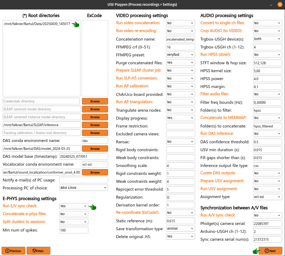
Neural recording data is aligned to the start of video recording, which is identifiable by searching for a ~2.3 s break in Loopbio Triggerbox pulses, which are constantly being transmitted to the Neuropixels digital input channel. The code recursively finds all the ap.bin files in the root directory and saves the digital input channel data (385th or last channel) to a separate Numpy file (which ends with _sync_ch_data.npy), if it hasn’t been saved already. After finding the tracking start and end (based on the largest Triggerbox break duration and total number of recording frames) in this Numpy file, the total video duration will then be compared to the total video-aligned neural recording, and you will get a report back whether that discrepancy is below 12 ms (in other words, less than 2 video frames, which is an acceptable level of distortion). Information at what Neuropixels sample the first and last video recording frame were detected will be saved to, for instance, /mnt/falkner/Bartul/EPHYS/20250430_imec0/changepoints_info_20250430_imec0.json, as exemplified below:
/mnt/falkner/Bartul/Data/:
├── 20250430_145017
│   ├── 20250430_145017_metadata.yaml
│   ├── audio
│   │   ...
│   ├── ephys
│   │   ├── imec0
│   │   │   ├── 20250430_145017.imec0.ap.bin
│   │   │   ├── 20250430_145017.imec0.ap.meta
│   │   │   ├── 20250430_145017_imec0_sync_ch_data.npy
│   │   ├── imec1
│   │       ├── 20250430_145017.imec1.ap.bin
│   │       ├── 20250430_145017.imec1.ap.meta
│   │       ├── 20250430_145017_imec1_sync_ch_data.npy
│   ├── sync
│   │   ...
│   │
│   └── video
│       ...
/mnt/falkner/Bartul/EPHYS:
├── 20250430_imec0
│   ├── changepoints_info_20250430_imec0.json
├── 20250430_imec1
│   ├── changepoints_info_20250430_imec1.json
In the changepoints JSON file, the E/V sync check process will save the tracking_start_end and largest_camera_break_duration values, and the latter, when divided with the Neuropixels sampling rate (should be ~30 kHz), should not be smaller than ~2.3 s.
"20250430_145017.imec0": {
    "session_start_end": [
        0,
        37825731
    ],
    "tracking_start_end": [
        850469,
        36867993
    ],
    "largest_camera_break_duration": 69341,
    "file_duration_samples": 37825731,
    "root_directory": "/mnt/falkner/Bartul/Data/20250430_145017",
    "total_num_channels": 385,
    "headstage_sn": "23280196",
    "imec_probe_sn": "22420015064"
}
The /usv-playpen/_parameter_settings/processing_settings.json file also contains a section not modifiable in the GUI itself, but it can be modified manually:
npx_file_type : Neuropixels 1.0 had “lf” and “ap” files, this field allows you to switch between them
npx_ms_divergence_tolerance : the maximum allowed difference between the video and e-phys recording duration in milliseconds; the default value is 12 ms but it can be tuned to whatever the user thinks is appropriate.
"validate_ephys_video_sync": {
        "npx_file_type": "ap",
        "npx_ms_divergence_tolerance": 12.0
}
Concatenate e-phys files
To run the concatenation of e-phys files (ap.bin), you need to list all the root directories of interest in order you want them to be concatenated, select Concatenate e-phys files, click Next and then Process:
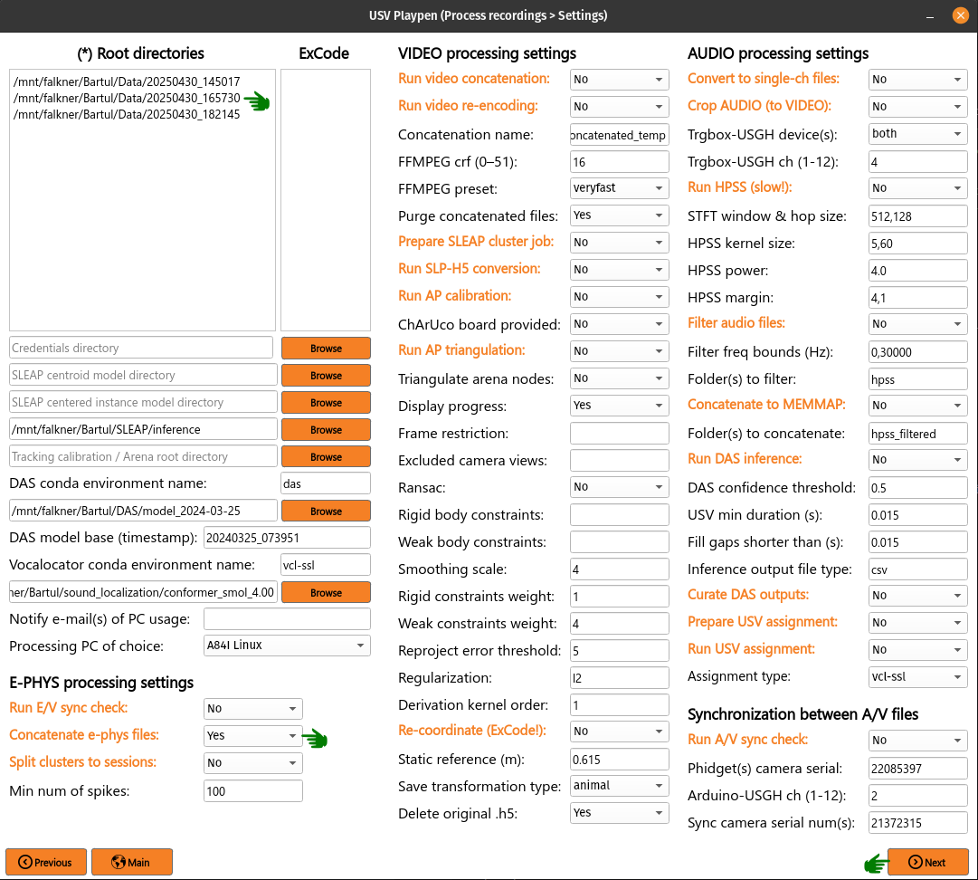
The code will find all the ap.bin files for each probe and conduct the concatenation to save the files in the EPHYS directory with the concatenated_ prefix:
/mnt/falkner/Bartul/Data/:
├── 20250430_145017
│   ├── 20250430_145017_metadata.yaml
│   ├── audio
│   │   ...
│   ├── ephys
│   │   ├── imec0
│   │   │   ├── 20250430_145017.imec0.ap.bin
│   │   │   ├── 20250430_145017.imec0.ap.meta
│   │   │   ├── 20250430_145017_imec0_sync_ch_data.npy
│   │   ├── imec1
│   │       ├── 20250430_145017.imec1.ap.bin
│   │       ├── 20250430_145017.imec1.ap.meta
│   │       ├── 20250430_145017_imec1_sync_ch_data.npy
│   ├── sync
│   │   ...
│   │
│   └── video
│       ...
/mnt/falkner/Bartul/EPHYS:
├── 20250430_imec0
│   ├── changepoints_info_20250430_imec0.json
│   ├── concatenated_20250430_imec0.ap.bin
├── 20250430_imec1
│   ├── changepoints_info_20250430_imec1.json
│   ├── concatenated_20250430_imec1.ap.bin
In the changepoints JSON file, the concatenation process will modify all lines other than the ones described above for E/V sync.
"20250430_145017.imec0": {
    "session_start_end": [
        0,
        37825731
    ],
    "tracking_start_end": [
        850469,
        36867993
    ],
    "largest_camera_break_duration": 69341,
    "file_duration_samples": 37825731,
    "root_directory": "/mnt/falkner/Bartul/Data/20250430_145017",
    "total_num_channels": 385,
    "headstage_sn": "23280196",
    "imec_probe_sn": "22420015064"
}
Split clusters to sessions
After spike sorting and post-sorting curation are complete, you can split the spikes of individual clusters back to the original sessions. To do this, even if you recorded multiple sessions in one day, it is sufficient to put only one root directory for that day, e.g., the first one. The script will find EPHYS root directory, and split spikes from all probes into sessions based on the inputs in the changepoints JSON file. Select Split clusters to sessions, click Next and then Process:
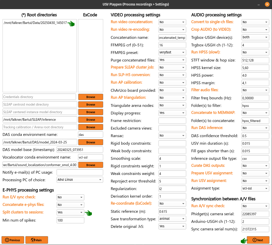
The code will create a cluster_data subdirectory in each session’s ephys/imec directory and populate it with Numpy files containing spike times in the shape of (2, number_of_spikes), where the first row contains spike times in seconds relative to start of tracking and the second row spike times according to what tracking frame they occurred in. Each cluster is named in the following format: probeID_clusterNumber_channelID_clusterType.npy.
├── 20250430_145017
│   ├── 20250430_145017_metadata.yaml
│   ├── audio
│   │   ...
│   ├── ephys
│   │   ├── imec0
│   │   │   ├── 20250430_145017.imec0.ap.bin
│   │   │   ├── 20250430_145017.imec0.ap.meta
│   │   │   ├── 20250430_145017_imec0_sync_ch_data.npy
│   │   │   ├── cluster_data
│   │   │   │   ├── imec0_cl0000_ch361_good.npy
│   │   │   │       ...
│   │   ├── imec1
│   │       ├── 20250430_145017.imec1.ap.bin
│   │       ├── 20250430_145017.imec1.ap.meta
│   │       ├── 20250430_145017_imec1_sync_ch_data.npy
│   │       ├── cluster_data
│   │       │   ├── imec1_cl0000_ch361_good.npy
│   │       │       ...
│   ├── sync
│   │   ...
│   │
│   └── video
│       ...
The /usv-playpen/_parameter_settings/processing_settings.json file also contains a section partially modifiable in the GUI, but it can entirely be modified manually:
min_spike_num : eliminate clusters with fewer spikes than this (set 0 if you want to keep all)
kilosort_version : Kilosort version in use
"get_spike_times": {
    "min_spike_num": 100,
    "kilosort_version": "4"
  },
Video processing
The processing of video data passes multiple stages:
Video concatenation and re-encoding (runs locally <20 min)
SLEAP inference (runs on cluster)
SLEAP proofreading (bottleneck step, requires extensive human curation)
SLP-H5 conversion (runs locally <1 min)
SLEAP-Anipose triangulation (runs locally <40 min)
Translate, rotate and scale SLEAP coordinates to metric units (runs locally <1 min)
Video concatenation and re-encoding
Before running this section, it is always a good idea to check that video files were copied to the file server correctly. These steps can be run separately (still in sequence, though), but for the sake of simplicity, they will be described jointly. To run video concatenation and re-encoding, you need to list the root directories of interest, select Run video concatenation and Run video re-encoding, click Next and then Process:
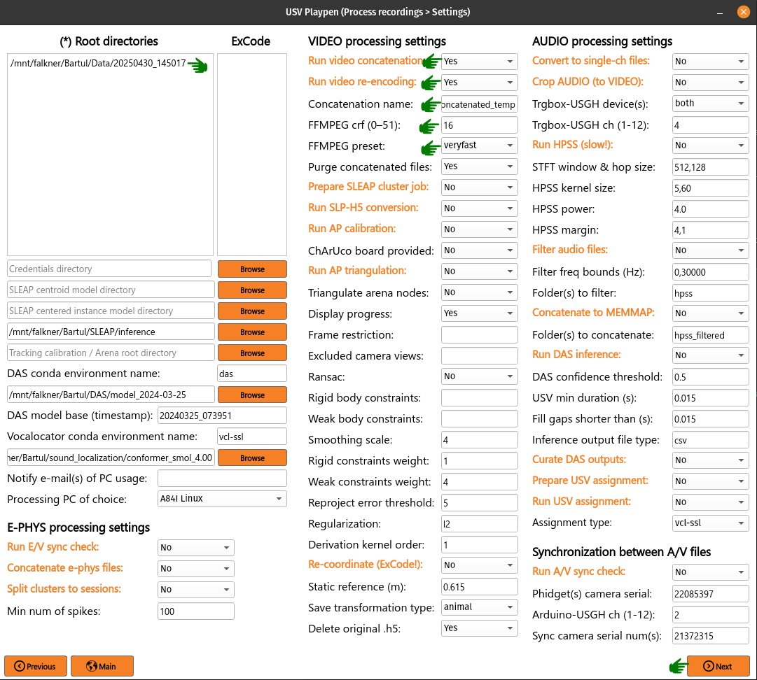
The re-encoding step will also result in the creation of the camera_frame_count_dict.json file, which contains numbers of frames for each camera in the session, as well as the total number of frames and video time for the camera with the least number of frames. The file will be saved in the video subdirectory of each session, and it will look like this:
{
"21241563": [
    180002,
    150.057
],
"21369048": [
    180000,
    150.057
],
"21372315": [
    180001,
    150.057
],
"21372316": [
    180001,
    150.056
],
"22085397": [
    180002,
    150.057
],
"total_frame_number_least": 180000,
"total_video_time_least": 1199.5477764606476,
"median_empirical_camera_sr": 150.057
}
These steps change videos and video directory structure from the native Loopbio format to one that is compatible with SLEAP-Anipose. Both rely on the usage of ffmpeg . After the steps are complete, the directory structure and file names should look as follows (displaying only one camera directory for brevity):
├── 20250430_145017
│   ├── 20250430_145017_metadata.yaml
│   ├── audio
│   │   ...
│   ├── ephys
│   │   ...
│   ├── sync
│   │   ...
│   │
│   └── video
│       ├── 20250430_145027.21241563
│       ...
│       ├── 20250430145035_camera_frame_count_dict.json
│       ├── 20250430145035
│       │    ├── 21241563
│       │    │   ├── calibration_images
│       │    │   ├── 21241563-20250430145035.mp4
│       ...
The /usv-playpen/_parameter_settings/processing_settings.json file also contains a section partially modifiable in the GUI, but it can entirely be modified manually:
concatenate_camera_serial_num / encode_camera_serial_num : serial numbers of cameras used in the recording (for concatenation / re-encoding, respectively)
concatenate_video_extension / encode_video_extension : video type (usually “mp4”)
concatenated_video_name : name of the concatenated video file
conversion_target_file : name of the concatenated video file as target for re-encoding
constant_rate_factor : FFMPEG constant rate factor for re-encoding
encoding_preset : FFMPEG encoding preset for re-encoding
delete_old_file : whether to delete the concatenated file after re-encoding
"concatenate_video_files": {
    "concatenate_camera_serial_num": [
      "21372315",
      "21372316",
      "21369048",
      "22085397",
      "21241563"
    ],
    "concatenate_video_extension": "mp4",
    "concatenated_video_name": "concatenated_temp"
  },
  "rectify_video_fps": {
    "encode_camera_serial_num": [
      "21372315",
      "21372316",
      "21369048",
      "22085397",
      "21241563"
    ],
    "conversion_target_file": "concatenated_temp",
    "encode_video_extension": "mp4",
    "constant_rate_factor": 16,
    "encoding_preset": "veryfast",
    "delete_old_file": true
  }
Prepare SLEAP cluster job
The usv-playpen GUI assumes usage of the SLEAP pose-tracking framework (SLEAP) for animal pose tracking. To do this, one first needs to train one or multiple models on the data of interest (i.e., social interactions). Explaining how to do this is beyond the scope of this text, so we will assume you already have a top-down centroid and centered instance model ready for running inference.
Since the average office PC does not necessarily have GPU-capabilities, it is advised to run SLEAP inference on a high-performance computing cluster, as these usually have GPU-capabilities and allow for the parallelization of the inference process. The usv-playpen GUI helps you prepare the SLEAP cluster job, but you will need to run the job on the cluster yourself.
The preparation consists of creating a job_list.txt file which contains the paths to the video files and the model(s) to be used for inference. The job list can then be used by a shell script, such as the one in /usv-playpen/other/cluster/SLEAP/sleap_inference_global.sh to execute inference on all video files of interest.
To run the SLEAP cluster job preparation, you need to list the root directories of interest (which will search for all videos recorded in those sessions), select the SLEAP conda environment name used on the cluster, select directories of centroid and centered instance models, select the output inference directory, select Make SLEAP job list, click Next and finally Process:
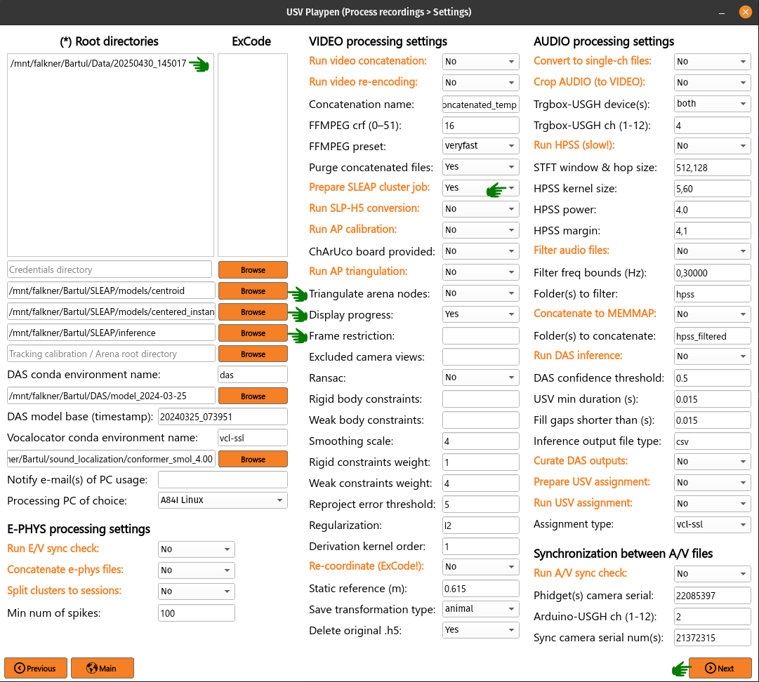
This shouldn’t take longer than several seconds - it will create/update the job_list.txt file in, for example, /mnt/falkner/Bartul/SLEAP/inference directory:
/mnt/falkner/Bartul/SLEAP/inference:
├── job_list.txt
│   ...
The /usv-playpen/_parameter_settings/processing_settings.json file contains a section partially modifiable in the GUI, but it can entirely be modified manually:
camera_names : camera serial numbers used in the recording
inference_root_dir : directory where the inference job list will be saved
centroid_model_path : path to the SLEAP centroid model
centered_instance_model_path : path to the SLEAP centered instance model
 "prepare_cluster_job": {
  "camera_names": [
    "21372315",
    "21372316",
    "21369048",
    "22085397",
    "21241563"
  ],
  "inference_root_dir": "/mnt/falkner/Bartul/SLEAP/inference",
  "centroid_model_path": "",
  "centered_instance_model_path": ""
}
SLEAP inference and proofreading
The SLEAP inference and proofreading steps are not implemented in the usv-playpen GUI. However, you can run the inference job on the cluster using the shell script mentioned above. The proofreading step is done in the SLEAP GUI, where it is crucial to correct identity switches and to keep the same animal identities across different video views. By current convention, that means the male mouse is always assigned identity 0, and the female mouse is always assigned identity 1.
Run SLP-H5 conversion
After proofreading, you convert SLP to H5 files, which is the format SLEAP-Anipose operates on (usv-playpen runs this in parallel for all views). To do this, you need to list the root directories of interest, select Run SLP-H5 conversion, click Next and then Process (NB: using the SLEAP uvx functionality, it is no longer necessary to install SLEAP to run this step):
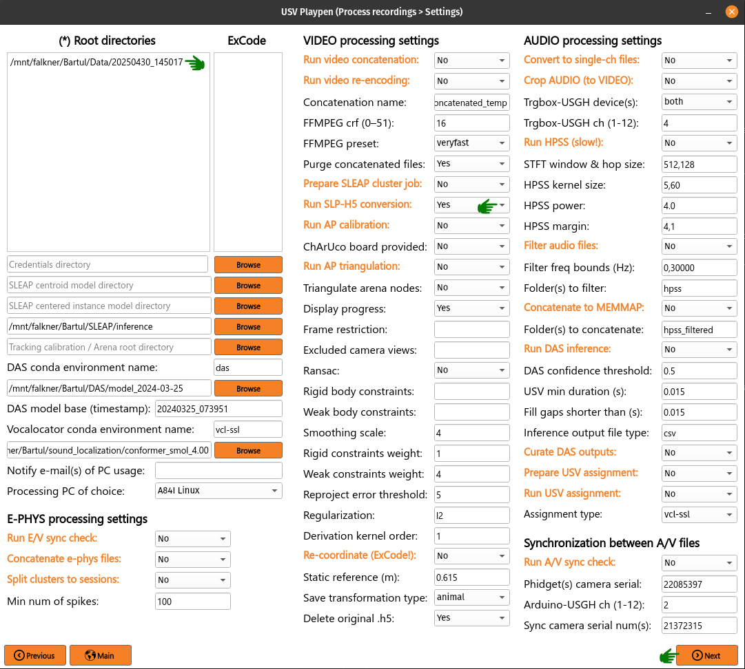
This step shouldn’t take longer than two minutes to run; the directory structure and file names should look as follows (displaying only one camera directory for brevity):
├── 20250430_145017
│   ├── 20250430_145017_metadata.yaml
│   ├── audio
│   │   ...
│   ├── ephys
│   │   ...
│   ├── sync
│   │   ...
│   │
│   └── video
│       ├── 20250430_145027.21241563
│       ...
│       ├── 20250430145035_camera_frame_count_dict.json
│       ├── 20250430145035
│       │    ├── 21241563
│       │    │   ├── calibration_images
│       │    │   ├── 21241563-20250430145035.h5
│       │    │   ├── 21241563-20250430145035.mp4
│       │    │   ├── 21241563-20250430145035.slp
│       ...
Run AP triangulation & Re-coordinate
Once SLP files are converted to H5, you are ready to run triangulation. Triangulation is the process of estimating the 3D coordinates of the tracked items based on the 2D coordinates from multiple camera views.
SLEAP-Anipose triangulation can be run to obtain 3D arena points, or 3D animal points.
3D arena points
It was previously explained how to record a calibration session, and in that session you recorded a 1-minute video of the arena with visible microphones and IR-reflective markers in its corners. All the video views of this recording can be loaded into the SLEAP GUI, and only on the first frame of each view, you label the 24 microphones and 4 corners with a 28-node skeleton that can be found in /usv-playpen/_config/playpen_skeleton.json. You label the microphones with the corresponding channel number, and corners with N, E, S and W, according to the following schematic:
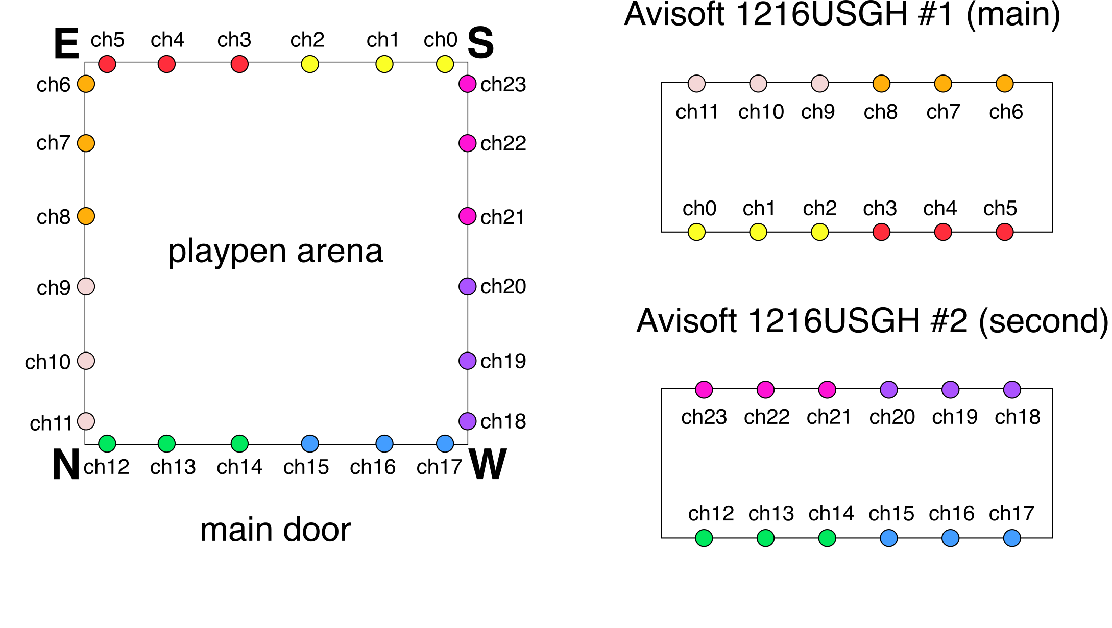
After labeling the first frame on each view, you can export the data as H5 files going to File > Export Analysis HDF5. You are now ready to run arena triangulation.
To do this, you need to list the root directories of interest, select the same root directory under Tracking calibration / arena root directory, select Run AP triangulation and Re-coordinate, select Triangulate arena nodes, select “arena” for Save transformation type and choose “No” for Delete original .h5. Finally, click Next and then Process:
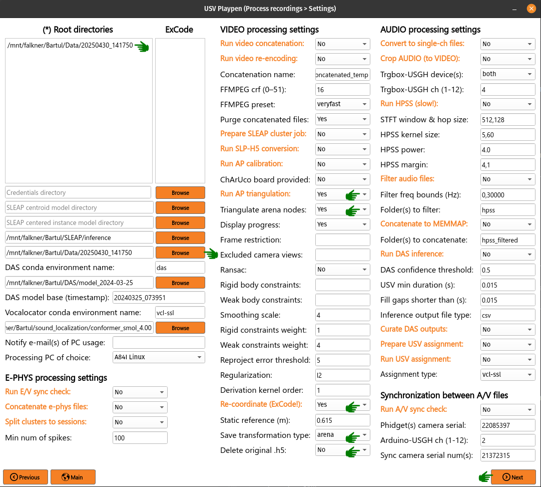
This shouldn’t take longer than one minute; the directory structure and file names should look as follows (note that you keep both the original and translated_rotated_metric H5 files!):
├── 20250430_145017
│   ...
│
├── 20250430_142022
│    ├── sync
│    │   ...
│    ├── video
│        ├── 20250430_142022.21241563
│        │   ...
│        ├── 20250430142022
│        │   ├── 20250430142022_points3d.h5
│        │   ├── 20250430142022_points3d_translated_rotated_metric.h5
│        │   ...
│        ├── calibration_20250430_141910.21241563
│        │   ...
3D animal points
To triangulate animal points, you need to list the root directories of interest, list their respective experimental codes, select the directory with the triangulated arena file, select Run AP triangulation and Re-coordinate, select “animal” for Save transformation type and choose “Yes” for Delete original .h5. Finally, click Next and then Process (a progress bar in the terminal will update you on the status of the process):
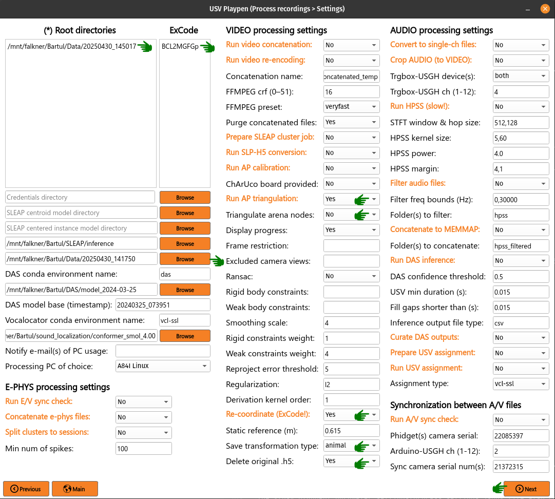
The process results in the creation of an H5 file which ends in _points3d_translated_rotated_metric.h5, and can be found as shown below:
├── 20250430_145017
│   ├── 20250430_145017_metadata.yaml
│   ├── audio
│   │   ...
│   ├── ephys
│   │   ...
│   ├── sync
│   │   ...
│   │
│   └── video
│       ├── 20250430_145027.21241563
│       ...
│       ├── 20250430145035_camera_frame_count_dict.json
│       ├── 20250430145035
│       │    ├── 20250430145035_points3d_translated_rotated_metric.h5
│       ...
The /usv-playpen/_parameter_settings/processing_settings.json file also contains a section partially modifiable in the GUI, but it can entirely be modified manually:
calibration_file_loc : directory containing the _calibration.toml file relevant for the session
triangulate_arena_points_bool : whether to triangulate arena or animal tracked nodes
frame_restriction : range of frames to be triangulated; empty finds the least number of frames across all cameras and triangulates those
excluded_views : list of camera serial numbers to be excluded from triangulation
display_progress_bool : whether to display the progress bar in the terminal during execution
ransac_bool : whether to use RANSAC for triangulation
rigid_body_constraints : list of rigid body constraints to be used for triangulation
weak_body_constraints : list of weak body constraints to be used for triangulation
smooth_scale : scale of the smoothing kernel
weight_weak : weight of the weak body constraints
weight_rigid : weight of the rigid body constraints
reprojection_error_threshold : threshold for reprojection error in pixels
regularization_function : regularization function to be used for triangulation
n_deriv_smooth : number of derivatives to be used for smoothing
original_arena_file_loc : directory containing the original arena 3D file
save_transformed_data : whether to save the transformed data as “animal” or “arena”
delete_original_h5 : whether to delete the original H5 file
static_reference_len : length of the static reference in meters, defaults to distance between two outer rail edges of two arena corners
experimental_codes : list of experimental codes associated with each session
"conduct_anipose_triangulation": {
  "calibration_file_loc": "",
  "triangulate_arena_points_bool": false,
  "frame_restriction": null,
  "excluded_views": [],
  "display_progress_bool": true,
  "ransac_bool": false,
  "rigid_body_constraints": [],
  "weak_body_constraints": [],
  "smooth_scale": 4,
  "weight_weak": 4,
  "weight_rigid": 1,
  "reprojection_error_threshold": 5,
  "regularization_function": "l2",
  "n_deriv_smooth": 1
},
"translate_rotate_metric": {
  "original_arena_file_loc": "",
  "save_transformed_data": "animal",
  "delete_original_h5": true,
  "static_reference_len": 0.615,
  "experimental_codes": []
}
The experimental codes are used to identify the session and the type of experiment conducted. The decoding sheet can be found below:
A - ablation
E - ephys
H - chemogenetics
O - optogenetics
P - playback
B - behavior
V - devocalization
U - urine/bedding

Q - alone
C - courtship
X - females
Y - males

L - light
D - dark

1,2,3 ... - number of animals

F - female
M - male

S - single
G - group

p - proestrus
e - estrus
m - metestrus
d - diestrus
Audio processing
The processing of audio data passes multiple stages:
Split audio to single files and crop to video duration (runs locally <15 min)
De-noise audio data with harmonic-percussive source separation (runs locally or on cluster)
Band-pass filter audio files (runs locally <15 min)
Concatenate all audio files to single MEMMAP file (runs locally <15 min)
Run DAS inference (runs on cluster)
Curate DAS outputs (runs locally <2 min)
Prepare USV assignment (runs locally <1 min)
Run USV assignment (runs locally <5 min)
Generate per-USV spectrograms (runs on cluster)
Generate USV masks — YOLO detection + SAM2 segmentation (runs on cluster)
Compute USV acoustic features (runs on cluster)
Infer QLVM latents and watershed categories (runs on cluster)
The QLVM decoder and mask detector that the last two steps rely on are trained separately, once per cohort — see Train spectrogram-pipeline models below.
Make mono and crop to video
Before running this section, it is always a good idea to check that audio files were copied to the file server correctly. These steps can be run separately (still in sequence, though), but for the sake of simplicity, they will be described jointly. To run these steps together, you need to list the root directories of interest, select Convert to single-ch files and Crop AUDIO (to VIDEO), click Next and then Process:
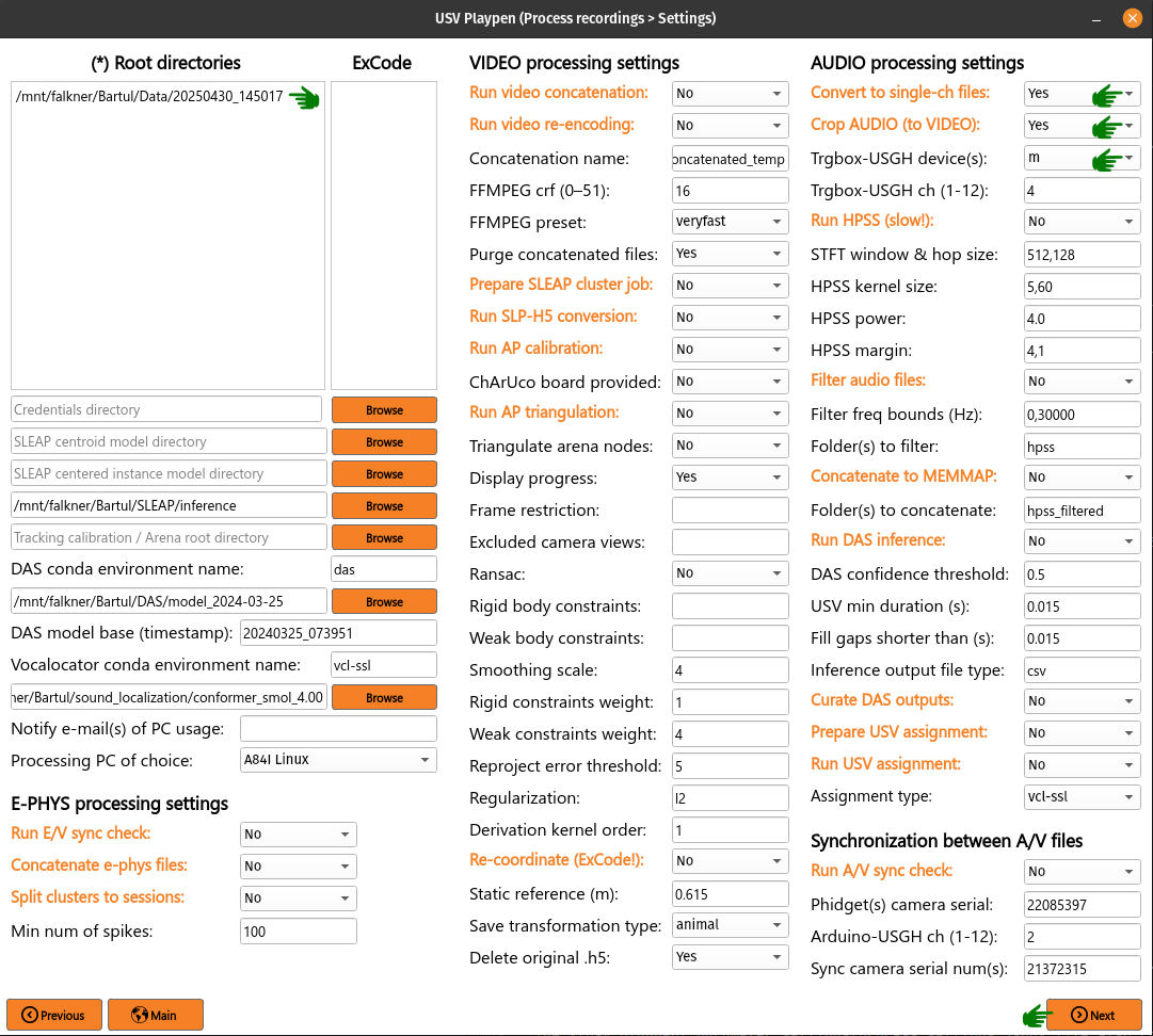
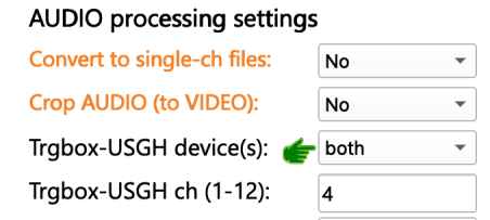
If you used the SYNC recording mode (usghflags: 1574), the Trgbox-USGH device(s) needs to be set to m. If you, however, used the NO SYNC recording mode (usghflags: 1862), the Trgbox-USGH device(s) needs to be set to both:
The Convert to single-ch files step populates the original directory with single channel files of the entire recording. The Crop AUDIO (to VIDEO) step will crop the audio files to the video duration, and save them in the cropped_to_video subdirectory. Both steps require the usage of sox. The original directory is later removed by the A/V sync check step (once synchronization passes the divergence tolerance), not by this step; reduced to one channel below for brevity:
├── 20250430_145017
│   ├── 20250430_145017_metadata.yaml
│   ├── audio
│   │   ├── cropped_to_video
│   │   │   ├── m_250430145009_ch01_cropped_to_video.wav
│   │   │       ...
│   │   ├── original_mc
│   │   │   ├── m_250430145009.wav
│   │   │       ...
│   │   ├── audio_triggerbox_sync_info.json
│   ├── ephys
│   │   ...
│   ├── sync
│   │   ├── m_video_frames_in_audio_samples.txt
│   │   ├── s_video_frames_in_audio_samples.txt
│   └── video
│       ...
The Crop AUDIO (to VIDEO) step will also result in the creation of a audio_triggerbox_sync_info.json file, which contains the sample number of first and last recorded video frame and the break duration detected prior to recording. It will also contain information about the total duration of the audio recording and its discrepancy with the duration of the video recording. In the sync subdirectory, the m_video_frames_in_audio_samples.txt and s_video_frames_in_audio_samples.txt files will be created, which contain the sample numbers of video frame starts in the audio recording. These files are useful should troubleshooting sync issues arise.
{
    "m": {
        "start_first_recorded_frame": 2654037,
        "end_last_recorded_frame": 302539204,
        "largest_break_duration": 578805,
        "duration_samples": 299885168,
        "duration_seconds": 1199.5407,
        "audio_tracking_diff_seconds": -0.0071,
        "num_dropouts": 0
    }
}
The /usv-playpen/_parameter_settings/processing_settings.json file contains a section fully modifiable in the GUI, with the following parameters:
device_receiving_input : USGH device receiving Loopbio Triggerbox input (if using SYNC mode, this should be “m”)
triggerbox_ch_receiving_input : microphone channel receiving Loopbio Triggerbox input
"crop_wav_files_to_video": {
    "device_receiving_input": "both",
    "triggerbox_ch_receiving_input": 4
  }
Run HPSS
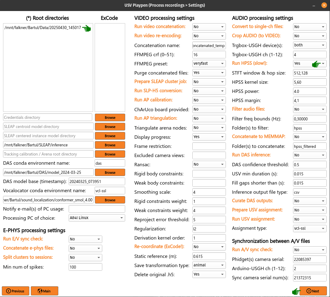
You have the option to denoise audio data using harmonic-percussive source separation (HPSS; implemented with librosa). You can find materials that allow you to run this analysis on the cluster in: /usv-playpen/other/cluster/HPSS. Alternatively, to run HPSS locally, you need to list the root directories of interest, select Run HPSS, click Next and then Process:
Below, you can see an example of an audio segment with mouse vocalizations before and after such denoising.
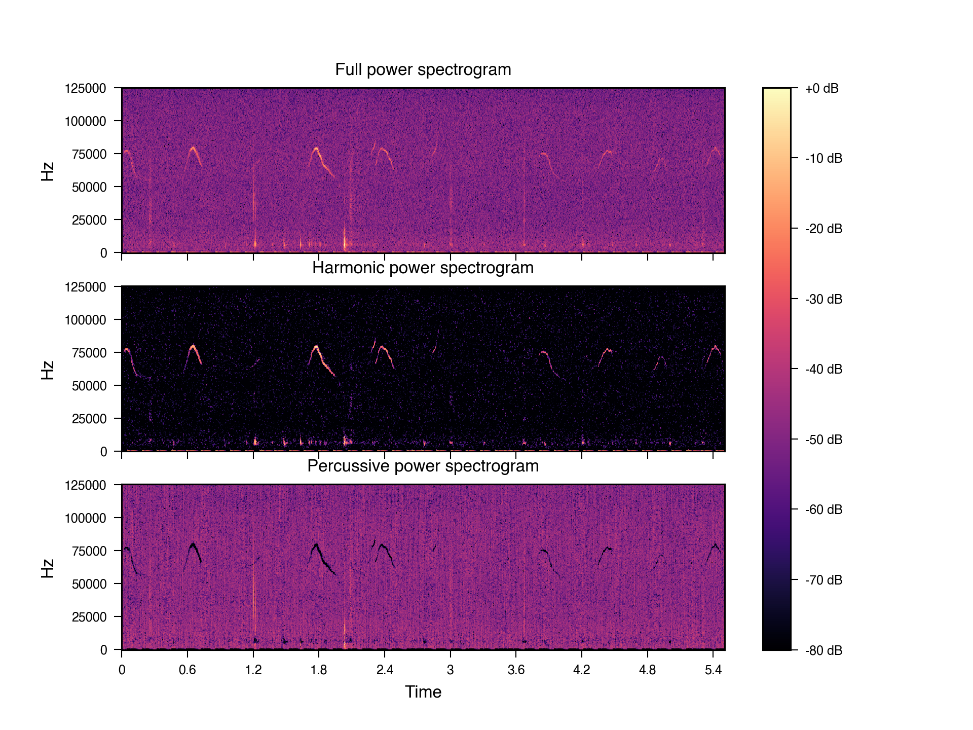
The Run HPSS step populates the hpss directory with de-noised single channel files of the entire recording (reduced to one channel for brevity):
├── 20250430_145017
│   ├── 20250430_145017_metadata.yaml
│   ├── audio
│   │   ├── cropped_to_video
│   │   │   ...
│   │   ├── hpss
│   │   │   ├── m_250430145009_ch01_cropped_to_video_hpss.wav
│   │   ├── original_mc
│   │   │   ...
│   │   ├── audio_triggerbox_sync_info.json
│   ├── ephys
│   │   ...
│   ├── sync
│   │   ...
│   └── video
│       ...
These four parameters are no longer exposed in the GUI (only the Run HPSS toggle remains); they are edited directly in the /usv-playpen/_parameter_settings/processing_settings.json file, under the following keys:
stft_window_length_hop_size : STFT window length and hop size
kernel_size : harmonic-percussive source separation kernel size
hpss_power : harmonic-percussive source separation power
margin : margin for harmonic-percussive source separation
"hpss_audio": {
    "stft_window_length_hop_size": [
      512,
      128
    ],
    "kernel_size": [
      5,
      60
    ],
    "hpss_power": 4.0,
    "margin": [
      4,
      1
    ]
}
Filter and concatenate to MEMMAP
These steps can be run separately (still in sequence, though), but for the sake of simplicity, they will be described jointly. To run these steps together, you need to list the root directories of interest, select Filter audio files and Concatenate to MEMMAP, click Next and then Process:
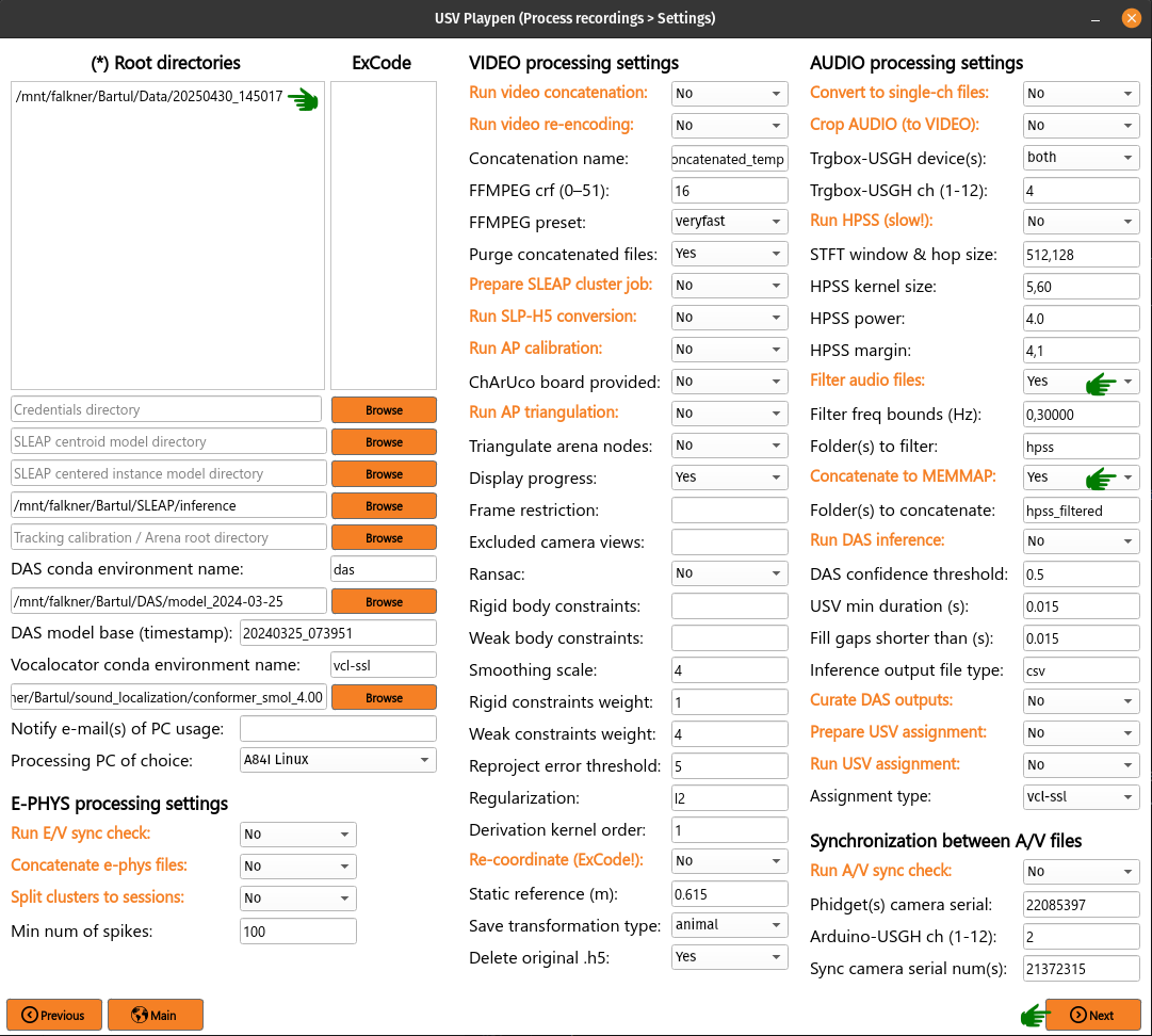
The purpose of these two functions is to first high-pass filter each audio file (removing all lower frequencies) and then concatenate all channels into one memory-mapped file. The first step requires the usage of sox. These processing steps populate the hpss_filtered directory with de-noised, high-pass filtered single channel files of the entire recording (reduced to one channel for brevity):
├── 20250430_145017
│   ├── 20250430_145017_metadata.yaml
│   ├── audio
│   │   ├── cropped_to_video
│   │   │   ...
│   │   ├── hpss
│   │   │   ...
│   │   ├── hpss_filtered
│   │   │   ├── 250430145009_concatenated_audio_hpss_filtered_250000_299885168_24_int16.mmap
│   │   │   ├── m_250430145009_ch01_cropped_to_video_hpss_filtered.wav
│   │   │   ...
│   │   ├── original_mc
│   │   │   ...
│   │   ├── audio_triggerbox_sync_info.json
│   ├── ephys
│   │   ...
│   ├── sync
│   │   ...
│   └── video
│       ...
The /usv-playpen/_parameter_settings/processing_settings.json file contains a section fully modifiable in the GUI, with the following parameters:
filter_audio_format : audio file format (usually “wav”)
filter_dirs : list of directories to be filtered (usually “hpss”)
filter_freq_bounds : frequency bounds for filtering (usually [0, 30000])
"filter_audio_files": {
    "filter_audio_format": "wav",
    "filter_dirs": [
      "hpss"
    ],
    "filter_freq_bounds": [
      0,
      30000
    ]
}
The Concatenate to MEMMAP step takes its parameters from the adjacent concatenate_audio_files block (also fully modifiable in the GUI):
concatenate_audio_format : audio file format to concatenate (usually “wav”)
concat_dirs : list of directories whose single-channel files are concatenated into the memory-mapped file (usually “hpss_filtered”)
"concatenate_audio_files": {
    "concatenate_audio_format": "wav",
    "concat_dirs": [
      "hpss_filtered"
    ]
}
Run DAS inference
The usv-playpen GUI assumes usage of the Deep Audio Segmenter (DAS) for identifying vocalizations in audio recordings. To do this, one first needs to train a model on the data of interest (i.e., social interactions with vocal output). Explaining how to do this is beyond the scope of this text, so we will assume you already have a model ready for running inference.
Since the average office PC does not necessarily have GPU-capabilities, it is advised to run DAS inference on a high-performance computing cluster, as these usually have GPU-capabilities and allow for the parallelization of the inference process. The usv-playpen GUI allows you to run the process locally (which can be time consuming), and it provides you with a shell script you can modify for cluster usage (/usv-playpen/other/cluster/DAS/das_inference_global.sh).
To run DAS inference, you need to list the root directories of interest, select the directory and base name of your DAS model, select Run DAS inference, click Next and finally Process:
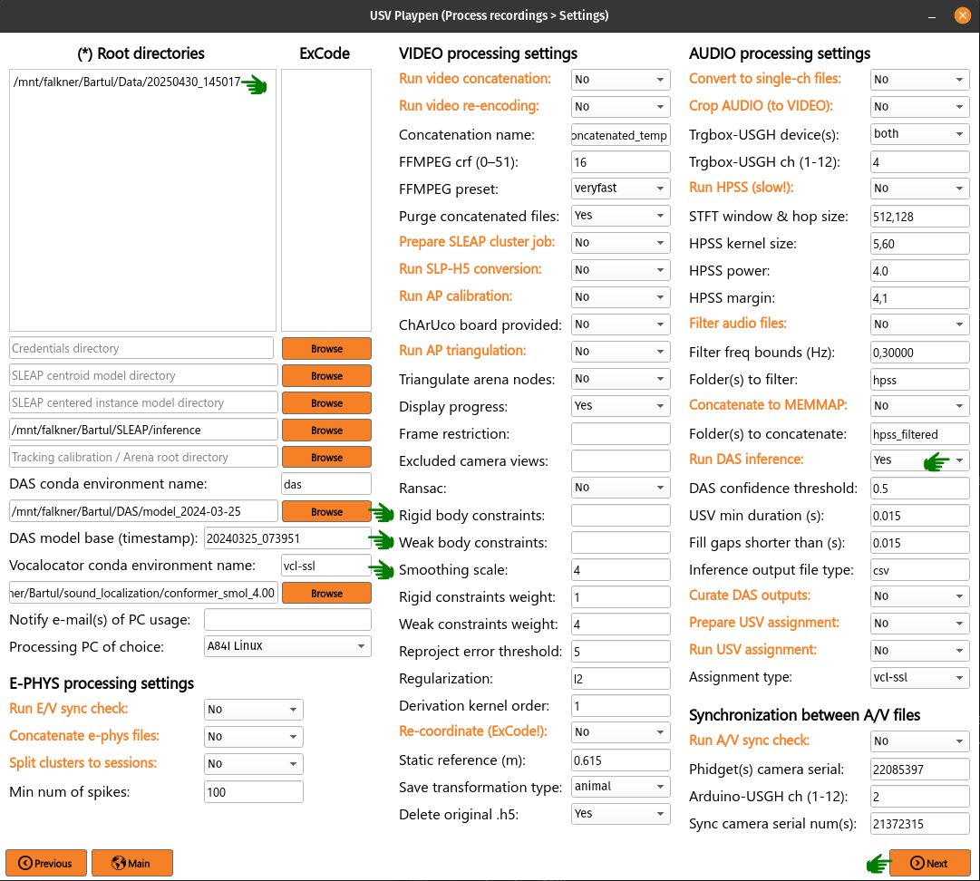
This will create a das_annotations subdirectory which will contain a CSV file for each recorded channel, denoting the start and end of each detected vocalization.
├── 20250430_145017
│   ├── 20250430_145017_metadata.yaml
│   ├── audio
│   │   ├── cropped_to_video
│   │   │   ...
│   │   ├── das_annotations
│   │   │   ├── m_250430145009_ch01_cropped_to_video_hpss_filtered_annotations.csv
│   │   │   ...
│   │   ├── hpss
│   │   │   ...
│   │   ├── hpss_filtered
│   │   │   ...
│   │   ├── original_mc
│   │   │   ...
│   │   ├── audio_triggerbox_sync_info.json
│   ├── ephys
│   │   ...
│   ├── sync
│   │   ...
│   └── video
│       ...
The /usv-playpen/_parameter_settings/processing_settings.json file contains a section partially modifiable in the GUI, but it can entirely be modified manually:
das_conda_env_name : name of the local conda environment used for running DAS inference (settings / CLI only; not exposed in the GUI)
das_model_directory : directory containing the trained DAS model
model_name_base : base name (date) of the trained DAS model
output_file_type : output file type (“csv” or “h5”)
segment_confidence_threshold : confidence threshold for segmenting vocalizations
segment_minlen : minimum length of segments to be considered vocalizations
segment_fillgap : maximum gap between segments to be joined into a single vocalization
"das_command_line_inference": {
    "das_conda_env_name": "das",
    "das_model_directory": "/mnt/falkner/Bartul/DAS/model_2024-03-25",
    "model_name_base": "20240325_073951",
    "output_file_type": "csv",
    "segment_confidence_threshold": 0.5,
    "segment_minlen": 0.015,
    "segment_fillgap": 0.015
  },
Curate DAS outputs
As explained above, DAS is run on every channel separately, such that a need arises to systematize different channel detections in one singular table. This code identifies the same detections across different channels and creates a single CSV file with the start and end times of each detected vocalization.
To run, you need to list the root directories of interest, select Curate DAS outputs, click Next and then Process:
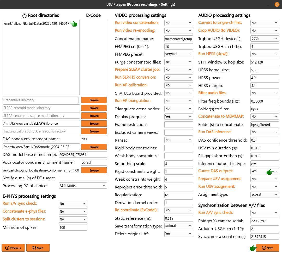
This process will create [1] a 20250430_145017_usv_summary.csv file, and [2] a 20250430_145017_usv_signal_correlation_histogram.svg file, as shown below:
├── 20250430_145017
│   ├── 20250430_145017_metadata.yaml
│   ├── audio
│   │   ├── cropped_to_video
│   │   │   ...
│   │   ├── das_annotations
│   │   │   ...
│   │   ├── hpss
│   │   │   ...
│   │   ├── hpss_filtered
│   │   │   ...
│   │   ├── original_mc
│   │   │   ...
│   │   ├── 20250430_145017_usv_summary.csv
│   │   ├── 20250430_145017_usv_signal_correlation_histogram.svg
│   │   ├── audio_triggerbox_sync_info.json
│   ├── ephys
│   │   ...
│   ├── sync
│   │   ...
│   └── video
│       ...
The usv_summary.csv file should look similar to an example table below:
┌────────┬─────────────┬─────────────┬──────────┬───┬─────────────┬───────────┬─────────────────────────────────┬──────────┐
│ usv_id ┆ start       ┆ stop        ┆ duration ┆ … ┆ mean_amp_ch ┆ chs_count ┆ chs_detected                    ┆ emitter  │
│ ---    ┆ ---         ┆ ---         ┆ ---      ┆   ┆ ---         ┆ ---       ┆ ---                             ┆ ---      │
╞════════╪═════════════╪═════════════╪══════════╪═══╪═════════════╪═══════════╪═════════════════════════════════╪══════════╡
│ 0      ┆ 0.23296     ┆ 0.299388    ┆ 0.066428 ┆ … ┆ 17.0        ┆ 24.0      ┆ [0, 1, 2, 3, 4, 5, 6, 7, 8, 9,… ┆ null     │
│ 1      ┆ 0.36064     ┆ 0.42278     ┆ 0.06214  ┆ … ┆ 17.0        ┆ 24.0      ┆ [0, 1, 2, 3, 4, 5, 6, 7, 8, 9,… ┆ null     │
│ 2      ┆ 0.488896    ┆ 0.58534     ┆ 0.096444 ┆ … ┆ 2.0         ┆ 24.0      ┆ [0, 1, 2, 3, 4, 5, 6, 7, 8, 9,… ┆ null     │
│ 3      ┆ 0.643392    ┆ 0.734588    ┆ 0.091196 ┆ … ┆ 2.0         ┆ 24.0      ┆ [0, 1, 2, 3, 4, 5, 6, 7, 8, 9,… ┆ null     │
│ 4      ┆ 0.800192    ┆ 0.942972    ┆ 0.14278  ┆ … ┆ 11.0        ┆ 24.0      ┆ [0, 1, 2, 3, 4, 5, 6, 7, 8, 9,… ┆ null     │
│ …      ┆ …           ┆ …           ┆ …        ┆ … ┆ …           ┆ …         ┆ …                               ┆ …        │
│ 2561   ┆ 1193.784896 ┆ 1193.828988 ┆ 0.044092 ┆ … ┆ 23.0        ┆ 20.0      ┆ [0, 1, 2, 3, 5, 6, 7, 8, 9, 11… ┆ null     │
│ 2562   ┆ 1195.412544 ┆ 1195.433852 ┆ 0.021308 ┆ … ┆ 23.0        ┆ 1.0       ┆ [23]                            ┆ null     │
│ 2563   ┆ 1195.531392 ┆ 1195.5639   ┆ 0.032508 ┆ … ┆ 23.0        ┆ 4.0       ┆ [0, 17, 21, 23]                 ┆ null     │
│ 2564   ┆ 1195.775552 ┆ 1195.81926  ┆ 0.043708 ┆ … ┆ 23.0        ┆ 24.0      ┆ [0, 1, 2, 3, 4, 5, 6, 7, 8, 9,… ┆ null     │
│ 2565   ┆ 1197.163712 ┆ 1197.196348 ┆ 0.032636 ┆ … ┆ 6.0         ┆ 2.0       ┆ [4, 6]                          ┆ null     │
└────────┴─────────────┴─────────────┴──────────┴───┴─────────────┴───────────┴─────────────────────────────────┴──────────┘
The usv_signal_correlation_histogram.svg file contains a histogram of [1] mean spectrogram correlations between channels and its noise/signal cutoff, and [2] the histogram of normalized spectral variance for single channel detections and its noise/signal cutoff (an example of which is shown below). The assumption is that noise correlates poorly across channels and has a smaller variance (as it is largely low volume).

The /usv-playpen/_parameter_settings/processing_settings.json file contains a section not modifiable in the GUI, but it can be modified manually:
filter_putative_noise_bool : whether to run the Phase-4 amplitude/spectrogram noise rejection; when
false, every merged detection is kept and the summary CSV is written as-is (peak/mean amplitude channels left at 0)len_win_signal : STFT window length
low_freq_cutoff : frequency cutoff for filtering (in Hz)
noise_corr_cutoff_min : minimum correlation coefficient for noise
noise_var_cutoff_max : maximum variance for noise
"summarize_das_findings": {
   "filter_putative_noise_bool": true,
   "len_win_signal": 512,
   "low_freq_cutoff": 30000,
   "noise_corr_cutoff_min": 0.15,
   "noise_var_cutoff_max": 0.001
}
Prepare and run USV assignment
You might also want to know which animal emitted which vocalization. To do this, usv-playpen relies on vocalocator, a tool for localizing animal vocalizations in 3D space, and it assumes you already have a trained model. These steps can be run separately (still in sequence, though), but for the sake of simplicity, they will be described jointly. To run these steps together, you need to list the root directories of interest, select the arena directory, select the directory of the vocalocator model, select Prepare USV assignment and Run USV assignment, select the Assignment type (vcl or vcl-ssl), click Next and then Process:
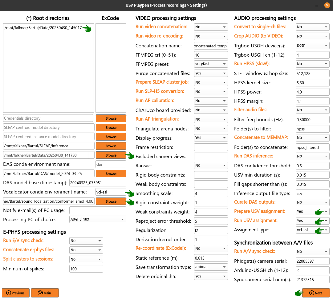
This will create a sound_localization subdirectory. With the default vcl-ssl backend, it contains a dset.h5 file (all data relevant for sound localization) and a model_predictions.npz file, whose predictions are transferred to the “emitter” column of the 20250430_145017_usv_summary.csv file. (With the older vcl backend it instead contains dset.h5, an assessment.h5 file with 2D assessment data, and an assessment_assn.npy file with 6D assessment output that feeds the “emitter” column.)
├── 20250430_145017
│   ├── 20250430_145017_metadata.yaml
│   ├── audio
│   │   ├── cropped_to_video
│   │   │   ...
│   │   ├── das_annotations
│   │   │   ...
│   │   ├── hpss
│   │   │   ...
│   │   ├── hpss_filtered
│   │   │   ...
│   │   ├── original_mc
│   │   │   ...
│   │   ├── sound_localization
│   │   │   ├── model_predictions.npz
│   │   │   ├── dset.h5
│   │   ├── 20250430_145017_usv_summary.csv
│   │   ├── 20250430_145017_usv_signal_correlation_histogram.svg
│   │   ├── audio_triggerbox_sync_info.json
│   ├── ephys
│   │   ...
│   ├── sync
│   │   ...
│   └── video
│       ...
The modified usv_summary.csv file now contains information in the last column for those vocalizations that have been attributed to specific animals:
┌────────┬─────────────┬─────────────┬──────────┬───┬─────────────┬───────────┬─────────────────────────────────┬──────────┐
│ usv_id ┆ start       ┆ stop        ┆ duration ┆ … ┆ mean_amp_ch ┆ chs_count ┆ chs_detected                    ┆ emitter  │
│ ---    ┆ ---         ┆ ---         ┆ ---      ┆   ┆ ---         ┆ ---       ┆ ---                             ┆ ---      │
│ i64    ┆ f64         ┆ f64         ┆ f64      ┆   ┆ f64         ┆ f64       ┆ str                             ┆ str      │
╞════════╪═════════════╪═════════════╪══════════╪═══╪═════════════╪═══════════╪═════════════════════════════════╪══════════╡
│ 0      ┆ 0.23296     ┆ 0.299388    ┆ 0.066428 ┆ … ┆ 17.0        ┆ 24.0      ┆ [0, 1, 2, 3, 4, 5, 6, 7, 8, 9,… ┆ null     │
│ 1      ┆ 0.36064     ┆ 0.42278     ┆ 0.06214  ┆ … ┆ 17.0        ┆ 24.0      ┆ [0, 1, 2, 3, 4, 5, 6, 7, 8, 9,… ┆ null     │
│ 2      ┆ 0.488896    ┆ 0.58534     ┆ 0.096444 ┆ … ┆ 2.0         ┆ 24.0      ┆ [0, 1, 2, 3, 4, 5, 6, 7, 8, 9,… ┆ 158114_2 │
│ 3      ┆ 0.643392    ┆ 0.734588    ┆ 0.091196 ┆ … ┆ 2.0         ┆ 24.0      ┆ [0, 1, 2, 3, 4, 5, 6, 7, 8, 9,… ┆ 158114_2 │
│ 4      ┆ 0.800192    ┆ 0.942972    ┆ 0.14278  ┆ … ┆ 11.0        ┆ 24.0      ┆ [0, 1, 2, 3, 4, 5, 6, 7, 8, 9,… ┆ 158114_2 │
│ …      ┆ …           ┆ …           ┆ …        ┆ … ┆ …           ┆ …         ┆ …                               ┆ …        │
│ 2561   ┆ 1193.784896 ┆ 1193.828988 ┆ 0.044092 ┆ … ┆ 23.0        ┆ 20.0      ┆ [0, 1, 2, 3, 5, 6, 7, 8, 9, 11… ┆ null     │
│ 2562   ┆ 1195.412544 ┆ 1195.433852 ┆ 0.021308 ┆ … ┆ 23.0        ┆ 1.0       ┆ [23]                            ┆ 156693_3 │
│ 2563   ┆ 1195.531392 ┆ 1195.5639   ┆ 0.032508 ┆ … ┆ 23.0        ┆ 4.0       ┆ [0, 17, 21, 23]                 ┆ null     │
│ 2564   ┆ 1195.775552 ┆ 1195.81926  ┆ 0.043708 ┆ … ┆ 23.0        ┆ 24.0      ┆ [0, 1, 2, 3, 4, 5, 6, 7, 8, 9,… ┆ null     │
│ 2565   ┆ 1197.163712 ┆ 1197.196348 ┆ 0.032636 ┆ … ┆ 6.0         ┆ 2.0       ┆ [4, 6]                          ┆ 156693_3 │
└────────┴─────────────┴─────────────┴──────────┴───┴─────────────┴───────────┴─────────────────────────────────┴──────────┘
The /usv-playpen/_parameter_settings/processing_settings.json file contains a section partially modifiable in the GUI, but it can entirely be modified manually:
vcl_conda_env_name : name of the local conda environment used for running Vocalocator (settings / CLI only; not exposed in the GUI)
vcl_model_directory : directory containing the trained Vocalocator model
vcl_version : version of the Vocalocator model (e.g., “vcl-ssl” for the SSL model)
"vocalocator": {
 "vcl_conda_env_name": "vcl-ssl-ss",
 "vcl_model_directory": "/mnt/falkner/Bartul/sound_localization/animal_id_model",
 "vcl_version": "vcl-ssl"
}
The assign_vocalizations block holds the confidence-set hyperparameters used
when turning the 6-D localizer output into per-mouse attributions (all exposed as
vcl-assign CLI flags):
temperature : covariance temperature scaling applied to the 6-D predictive covariance.
grid_resolution : spatial
(x_res, y_res)grid the confidence-set PDF is sampled on. The same grid drives both the PDF construction and the point-in-set lookup, so it is a single shared value.n_angle_bins : number of angular histogram bin edges (
-pitopi).n_samples : Monte-Carlo sample count for the per-vocalization angle PDF.
confidence_level : confidence level (in
[0, 1]) for the extracted confidence sets.angle_pdf_seed : RNG seed for the reproducible angle-PDF sampling.
"assign_vocalizations": {
 "temperature": 1.0,
 "grid_resolution": [100, 100],
 "n_angle_bins": 46,
 "n_samples": 500,
 "confidence_level": 0.95,
 "angle_pdf_seed": 0
}
Render spectrograms and latents
Once the curated usv_summary.csv exists (see Curate DAS outputs above), an in-house, self-contained pipeline turns every detected ultrasonic vocalization (USV) into a spectrogram, a USV mask, interpretable acoustic features, and toroidal QLVM latents. These steps can be run separately (still in sequence, though), but for the sake of simplicity, they will be described jointly. To run them together, you need to list the root directories of interest, set the Spectrogram models directory (the single root from which the Segment Anything Model 2 (SAM2), YOLO, and QLVM model paths are derived), select Generate spectrograms, Generate masks, Compute USV features and Infer QLVM latents, click Next and then Process (GPU is required):
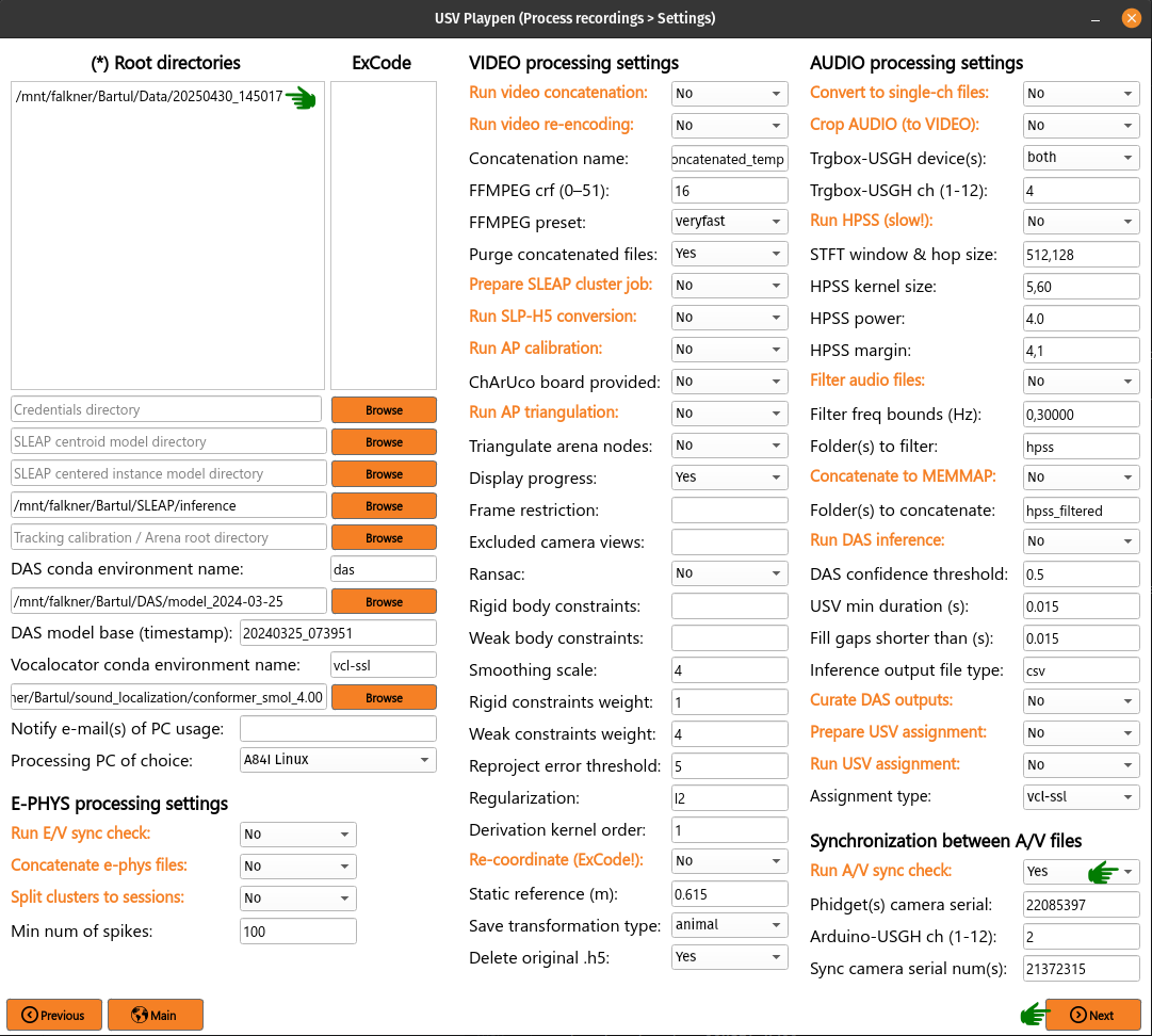
The Generate spectrograms step computes a variance-weighted, multi-channel spectrogram of every USV; Generate masks runs a YOLO box detector and prompts SAM2 to segment each call; Compute USV features derives per-USV spectral and amplitude features; and Infer QLVM latents embeds each spectrogram into the trained QLVM torus and assigns it a vocal category. The mask and latent steps run on the GPU and rely on two pre-trained models (see Train spectrogram-pipeline models below). The spectrogram and mask arrays are written to a new spectrograms subdirectory, while the acoustic features and QLVM latents are merged into usv_summary.csv:
├── 20250430_145017
│   ├── 20250430_145017_metadata.yaml
│   ├── audio
│   │   ├── cropped_to_video
│   │   │   ...
│   │   ├── das_annotations
│   │   │   ...
│   │   ├── hpss
│   │   │   ...
│   │   ├── hpss_filtered
│   │   │   ...
│   │   ├── original_mc
│   │   │   ...
│   │   ├── sound_localization
│   │   │   ...
│   │   ├── spectrograms
│   │   │   ├── 20250430_145017_spectrograms.h5
│   │   ├── 20250430_145017_usv_summary.csv
│   │   ├── audio_triggerbox_sync_info.json
│   ├── ephys
│   │   ...
│   ├── sync
│   │   ...
│   └── video
│       ...
The 20250430_145017_spectrograms.h5 file holds the spectrograms (created by Generate spectrograms) and the masks (appended by Generate masks), grouped per session:
20250430_145017_spectrograms.h5
├── frequency_bins (F,)                                  # Generate spectrograms
├── spectrogram/20250430_145017/spectrograms (N, F, T)   # Generate spectrograms
├── spectrogram/20250430_145017/durations (N,)           # Generate spectrograms
├── mask/20250430_145017/segmentations (M, F, T) bool    # Generate masks
└── mask/20250430_145017/spectrogram_index (M,)          # Generate masks
The spectrogram rows are 1:1 with usv_summary.csv; each mask row carries a spectrogram_index pointing back to the spectrogram (and USV) it segments. Re-running a step overwrites only the group it owns and leaves the rest of the file intact.
The Compute USV features and Infer QLVM latents steps add columns to usv_summary.csv in place. Compute USV features adds:
mean_freq_hz : energy-weighted mean frequency of the USV (Hz)
peak_freq_hz : frequency of peak energy (Hz)
freq_bandwidth_hz : spectral bandwidth between the low/high cumulative-energy edges (Hz)
mean_amplitude : mean spectrogram amplitude over the USV (a.u.)
max_amplitude : maximum spectrogram amplitude over the USV (a.u.)
spectral_entropy : spectral entropy of the USV (nats)
┌────────┬───┬──────────────┬──────────────┬───────────────────┬────────────────┬───────────────┬──────────────────┐
│ usv_id ┆ … ┆ mean_freq_hz ┆ peak_freq_hz ┆ freq_bandwidth_hz ┆ mean_amplitude ┆ max_amplitude ┆ spectral_entropy │
│ ---    ┆   ┆ ---          ┆ ---          ┆ ---               ┆ ---            ┆ ---           ┆ ---              │
│ i64    ┆   ┆ f64          ┆ f64          ┆ f64               ┆ f64            ┆ f64           ┆ f64              │
╞════════╪═══╪══════════════╪══════════════╪═══════════════════╪════════════════╪═══════════════╪══════════════════╡
│ 0      ┆ … ┆ 68421.3      ┆ 71250.0      ┆ 24180.5           ┆ 0.182          ┆ 0.94          ┆ 0.61             │
│ 1      ┆ … ┆ 72980.1      ┆ 75000.0      ┆ 18640.2           ┆ 0.211          ┆ 0.88          ┆ 0.55             │
│ …      ┆ … ┆ …            ┆ …            ┆ …                 ┆ …              ┆ …             ┆ …                │
└────────┴───┴──────────────┴──────────────┴───────────────────┴────────────────┴───────────────┴──────────────────┘
Infer QLVM latents adds:
qlvm_dim1 / qlvm_dim2 : the two torus (latent) coordinates
qlvm_category : the FINE watershed cluster label (vocal category)
qlvm_supercategory : the COARSE watershed cluster label (
0= background / noise)
┌────────┬───┬───────────┬───────────┬───────────────┬────────────────────┐
│ usv_id ┆ … ┆ qlvm_dim1 ┆ qlvm_dim2 ┆ qlvm_category ┆ qlvm_supercategory │
│ ---    ┆   ┆ ---       ┆ ---       ┆ ---           ┆ ---                │
│ i64    ┆   ┆ f64       ┆ f64       ┆ i64           ┆ i64                │
╞════════╪═══╪═══════════╪═══════════╪═══════════════╪════════════════════╡
│ 0      ┆ … ┆ 0.4123    ┆ 0.8871    ┆ 7             ┆ 3                  │
│ 1      ┆ … ┆ 0.1902    ┆ 0.3320    ┆ 2             ┆ 1                  │
│ …      ┆ … ┆ …         ┆ …         ┆ …             ┆ …                  │
└────────┴───┴───────────┴───────────┴───────────────┴────────────────────┘
These columns are comparable across every session embedded into the same QLVM model, and are consumed by the categorical USV-tuning analysis in Analyze (Compute neuronal tuning curves). When a mask is present for a call, the acoustic features are computed over the true SAM mask region; otherwise they fall back to the signal time-window.
The /usv-playpen/_parameter_settings/processing_settings.json file contains the settings for these steps, partially modifiable in the GUI but fully modifiable manually. The six SAM2 / YOLO / QLVM model paths all derive from a single spectrograms_root (GUI: Spectrogram models directory): set that one directory and the paths below are filled as <root>/sam/... and <root>/qlvm/.... Set any individual path explicitly (in the JSON or via a CLI flag) to override its derived default; generate_masks.sam2_model_cfg is a config name, not a path, so it is never derived.
"spectrograms_root": "/mnt/falkner/Bartul/spectrograms"
Generate spectrograms (generate_spectrograms):
num_freq_bins : number of spectrogram frequency bins (output height)
num_time_bins : number of spectrogram time bins (output width)
nperseg : STFT window length / n_fft (samples)
noverlap : legacy scipy-style STFT overlap kept for parity with the QLVM training config; it is not used to compute the spectrogram (the hop is governed by
hop_length)min_freq : lower frequency cutoff (Hz)
max_freq : upper frequency cutoff (Hz)
hop_length : STFT hop length (samples; defaults to
nperseg // 4when null)window : STFT window function
offset : time padding added before each USV onset and after each offset (seconds)
normalize : whether to min-max normalize each spectrogram to [0, 1]
"generate_spectrograms": {
    "num_freq_bins": 128,
    "num_time_bins": 128,
    "nperseg": 2048,
    "noverlap": 1792,
    "min_freq": 30000,
    "max_freq": 120000,
    "hop_length": 512,
    "window": "blackmanharris",
    "offset": 0.0,
    "normalize": true
  }
Generate masks (generate_masks):
method : mask-generation method (
boxprompt= box-prompted SAM2 segmentation)detector : box detector backend (
yololearned detector orccconnected-component baseline)sam2_model_dir : SAM2 model directory (config/checkpoint resolve against it; the step changes into it)
sam2_model_cfg : SAM2 config name/path (resolved from the SAM2 install’s Hydra search path)
sam2_model_path : SAM2 checkpoint path
yolo_weights : trained YOLO
best.ptweights pathyolo_conf : YOLO confidence threshold (lower → more recall)
yolo_iou : YOLO NMS IoU (raise to keep stacked calls)
yolo_imgsz : YOLO inference image size (px)
mask_cmap : colormap used to render each spectrogram to RGB before detection
duration_min : minimum USV duration (time bins) to segment; shorter rows are skipped
batch_size : number of spectrograms per SAM2 batch
multimask_output : whether SAM2 returns multiple candidate masks per box (the best is kept)
iou_floor : minimum SAM2 predicted-IoU quality for a mask
drop_below_iou : if true, drop masks below
iou_floor(else keep)split_disconnected : split a mask with disconnected components into separate instances
max_iters : maximum SAM2 prompt-refinement iterations per box
merge_instances : merge overlapping per-box mask instances
merge_iou : IoU above which two instances are merged
merge_containment : containment fraction above which one instance is absorbed into another
mask_intensity_floor : minimum normalized spectrogram intensity for a pixel to remain in a mask
tiny_mask_floor_px : drop masks smaller than this many pixels
min_box_area : drop detector boxes smaller than this area (px²; 0 disables)
"generate_masks": {
    "method": "boxprompt",
    "detector": "yolo",
    "sam2_model_dir": "",
    "sam2_model_cfg": "configs/sam2.1/sam2.1_hiera_b+.yaml",
    "sam2_model_path": "",
    "yolo_weights": "",
    "yolo_conf": 0.25,
    "yolo_iou": 0.7,
    "yolo_imgsz": 128,
    "mask_cmap": "viridis",
    "duration_min": 10,
    "batch_size": 12,
    "multimask_output": true,
    "iou_floor": 0.7,
    "drop_below_iou": false,
    "split_disconnected": true,
    "max_iters": 1,
    "merge_instances": true,
    "merge_iou": 0.5,
    "merge_containment": 0.8,
    "mask_intensity_floor": 0.0,
    "tiny_mask_floor_px": 12,
    "min_box_area": 0
  }
When left empty (the default) the SAM2/YOLO paths are derived from spectrograms_root above; whether derived or set explicitly, they are stored in the canonical /mnt/falkner/... lab-share form and translated to the host’s mount root (e.g. /Volumes/falkner on macOS) via configure_path, the same handling as the DAS / Vocalocator model paths. sam2_model_cfg is a config name resolved inside the SAM2 install, not a mount path. Both sam2 and ultralytics (usv-playpen core dependencies) must be installed.
Compute USV features (compute_usv_acoustic_features):
low_energy_frac : lower edge of the cumulative-energy band used for spectral bandwidth
high_energy_frac : upper edge of the cumulative-energy band used for spectral bandwidth
"compute_usv_acoustic_features": {
    "low_energy_frac": 0.05,
    "high_energy_frac": 0.95
  }
Infer QLVM latents (infer_qlvm_latents):
weights_npz_path : path to the QLVM decoder weights
.npz(written by Train QLVM)reference_arrays_fine_npz_path : path to the FINE reference
arrays.npz(itsws_labels_periodicgrid →qlvm_category)reference_arrays_coarse_npz_path : path to the COARSE reference
arrays.npz(itsws_labels_periodicgrid →qlvm_supercategory)lattice_type : quasi-random lattice generator (must match training)
latent_dim : torus latent dimensionality (must match training)
n_points : number of lattice points (must match training)
korobov_a : Korobov generating integer (must match training)
fib_m : Fibonacci lattice parameter (must match training)
time_stretch : whether to time-stretch spectrograms before embedding (must match training)
masking_type :
"sam"(default) masks each spectrogram by the union of its SAM regions before embedding, matching how the decoder was trained by Build QLVM training set;"none"embeds raw spectrograms (must match training)target_shape : output spectrogram
(freq, time)shape the embedder resizes to before inference; must match thetarget_shapeused by Build QLVM training set (default[128, 128])
"infer_qlvm_latents": {
    "weights_npz_path": "",
    "reference_arrays_fine_npz_path": "",
    "reference_arrays_coarse_npz_path": "",
    "lattice_type": "korobov",
    "latent_dim": 2,
    "n_points": 1021,
    "korobov_a": 76,
    "fib_m": 16,
    "time_stretch": false,
    "masking_type": "sam",
    "target_shape": [128, 128]
  }
Train spectrogram-pipeline models
Two per-session inference steps lean on learned models: Generate (spectrogram) masks uses a detector to find each USV, and Infer QLVM latents uses a decoder to embed it. Both are trained once on a representative cohort and then reused for every future session — so this is a setup / maintenance step, not part of routine per-experiment processing. Retrain only when something changes materially: a new or substantially expanded cohort, a different spectrogram representation, or revised category definitions.
Both train cross-session via CLI / cluster commands only (no GUI buttons): each is a two-command chain over a comma-separated list of session --root-directories writing standalone artifacts to --output-directory. SAM2 is used pretrained — it is not trained here. Full flags for CLI can be found here.
QLVM decoder
Defines the shared toroidal latent space (and watershed categories) that makes the qlvm_* columns comparable across every session embedded with the same model. build-qlvm-training-set aggregates the cohort’s *_spectrograms.h5 into a curated set (--masking-type sam masks each spectrogram by its SAM region, the default; none keeps raw spectrograms) → train_data.npz + val_data.npz (or full_data.npz) + metadata.npz. train-qlvm then trains the decoder → qmc_train_qlvm.tar + qmc_decoder_weights.npz (reloaded by infer-qlvm-latents). Cluster submitter: train_qlvm_global.sh.
Mask detector
The YOLO box detector that localizes each call in its spectrogram so SAM2 can segment it; generate-usv-masks reloads its weights. export-yolo-dataset renders the cohort’s spectrograms to an Ultralytics dataset (images/ + labels/ + data.yaml); train-masks fine-tunes YOLO → the run directory + best.pt. Cluster submitter: train_masks_global.sh.
Box labels are set by --label-source (or export_yolo_dataset.label_source): cc (default — pseudo-labels from the connected-component detector; zero manual work, no GPU; the recommended start), manual (hand-verified {spec_id}.txt YOLO files in --manual-labels-directory), or merge (cc pseudo-labels overridden by manual files where present). manual / merge require --manual-labels-directory; cc ignores it. The submitter exposes a LABEL_SOURCE knob and MANUAL_LABELS_DIRECTORY. Both generate-usv-masks and train-masks need the sam2 and ultralytics packages (usv-playpen core dependencies).
A/V synchronization
To run audio/video (A/V) synchronization, you need to list the root directories of interest, select Run A/V sync check, click Next and then Process:
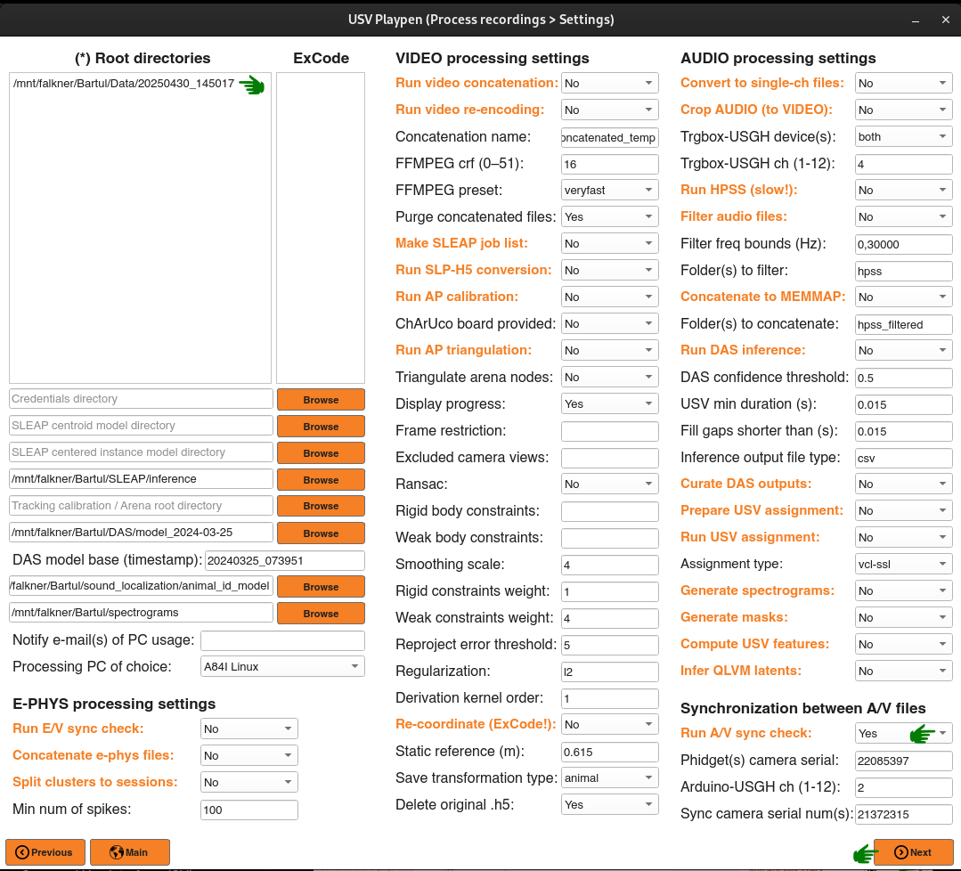
The A/V synchronization procedure will first create a sync_px file for each input camera, recording pixel intensities of each LED position. The objective is to identify the start of each IPI event in camera time and on both audio devices. One can then compare, for each individual IPI event, what the discrepancy is between the clocks of both devices and that is captured in the summary.svg histograms.
├── 20250430_145017
│   ├── 20250430_145017_metadata.yaml
│   ├── audio
│   │   ...
│   ├── ephys
│   │   ...
│   ├── sync
│   │   ...
│   │   ├── nidq_ipi_data.npy
│   │   ├── sync_px_21372315-250430145009
│   │   ├── 20250430_145017_summary.svg
│   └── video
│       ...
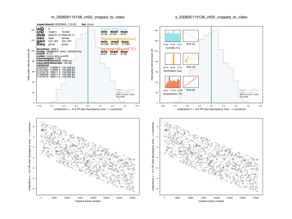
An example output of the A/V synchronization procedure is shown below.
Notice that the plot contains two columns, one for each Avisoft UltraSoundGate hardware (USGH) device (which can operate in NO SYNC mode). In the first row, you can observe the distribution of A-V IPI discrepancies, which is the difference between the IPI onsets detected in the video and audio data. In the example, you can see the discrepancy goes rarely beyond one camera frame, which is ~6 ms, an acceptable amount of jitter. One might also be interested in viewing how this discrepancy evolves over time. One thing we would want to avoid are drastic changes in sampling rates on any of the devices over time. In the second row, you can see the relationship between IPI onsets time (earlier-later in the session) and the A-V IPI discrepancy. Ideally, we would want to observe a flat cloud of points, which would indicate that the A/V IPI discrepancy is stable over time. If you observe a trend that goes beyond 2 tracking frames, it might be worth investigating further.
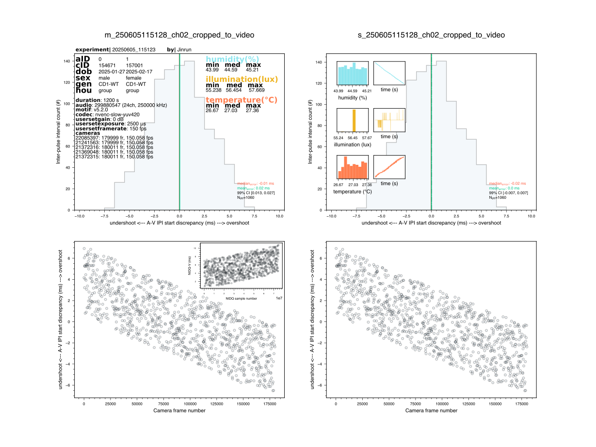
In case NIDQ was also used in the recording, the first of the device plots will have a subplot detailing the temporal relationship between the NIDQ IPI onsets and the video IPI onsets (in ms). This plot is informative in case there is a large A-V discrepancy, as it allows you to determine which device (A or V) is having issues. If the NIDQ-V discrepancy is small, the sync issue is likely related to the audio device. On the contrary, if the NIDQ-V discrepancy is large, the sync issue is likely related to the video device. Either way, this is a first step in investigating this further, which is highly recommended.
The /usv-playpen/_parameter_settings/processing_settings.json file contains a section fully modifiable in the GUI, with the following parameters:
extra_data_camera : serial number of the camera used to store phidget data
sync_ch_receiving_input : microphone channel receiving Arduino digital input
extract_exact_video_frame_times_bool : instead of using frame indices multiplied by empirical frame rate, use Loopbio times directly (which is less precise!)
nidq_sr : sampling rate of the NIDQ device (in Hz)
nidq_num_channels : number of channels on the NIDQ device (9 on BNC-2110)
nidq_bool : whether NIDQ device received Triggerbox AND sync input
nidq_triggerbox_input_bit_position : triggerbox input bit position on the NIDQ device digital channel (assumes last channel is digital!)
nidq_sync_input_bit_position : sync input bit position on the NIDQ device digital channel (assumes last channel is digital!)
sync_camera_serial_num : serial numbers of cameras that can detect flashing LEDs
led_px_version : version of the LED pixel positions
led_px_dev : maximal deviation (in px) of observed LED flashes relative to expected positions
sync_video_extension : video type (usually “mp4”)
relative_intensity_threshold : top threshold (on 0-1 scale) for relative temporal change in pixel intensity
millisecond_divergence_tolerance : maximal deviation of IPI onsets (in ms) between video detections and ground truth
"extract_phidget_data": {
 "Gatherer": {
   "prepare_data_for_analyses": {
     "extra_data_camera": "22085397"
   }
 }
},
"find_audio_sync_trains": {
     "sync_ch_receiving_input": 2,
     "extract_exact_video_frame_times_bool": false,
     "nidq_sr": 62500.72887,
     "nidq_num_channels": 9,
     "nidq_bool": false,
     "nidq_triggerbox_input_bit_position": 5,
     "nidq_sync_input_bit_position": 7
 },
"find_video_sync_trains": {
     "sync_camera_serial_num": [
         "21372315"
     ],
     "led_px_version": "current",
     "led_px_dev": 10,
     "sync_video_extension": "mp4",
     "relative_intensity_threshold": 1.0,
     "millisecond_divergence_tolerance": 12
}