Visualize
This page explains how to use the data visualization functionalities in the usv-playpen GUI:
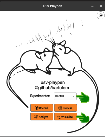
In order to run any of the functions detailed below, select an experimenter name from the dropdown menu and click the Visualize button on the GUI main display:
Clicking the Visualize button will open a new window with all the offered functionalities (see below):
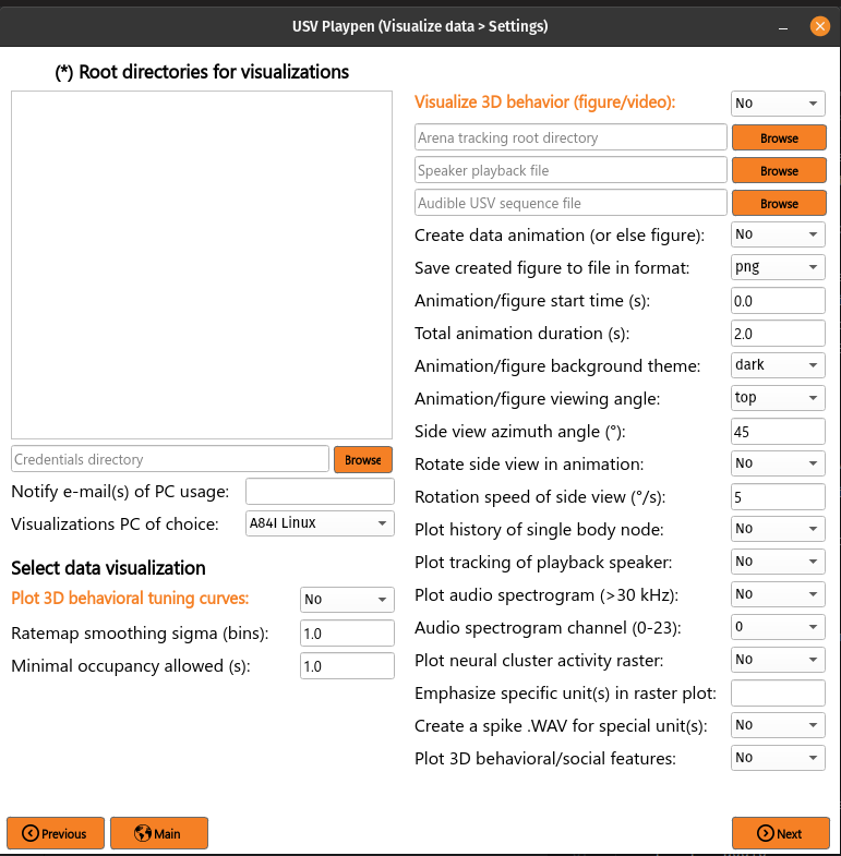
All the main functions are outlined in orange, and black fields are function-specific options tunable by the user in the GUI. It is important to note that these are not necessarily all the options the user can set, and the full list of options can be found under each function in the /usv-playpen/_parameter_settings/visualizations_settings.json file. Each time the user clicks the Next button in the window above, visualizations_settings.json is modified to the newest input configuration.
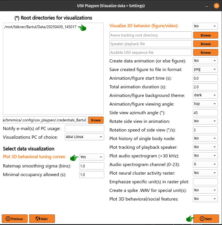
The Root directories field enables you to list the directories containing the data you want to visualize. Each root directory should be in its own row; for example, three sessions should be listed as follows:
F:\Bartul\Data\20250430_145017
F:\Bartul\Data\20250430_165730
F:\Bartul\Data\20250430_182145
Plot neuronal tuning figures
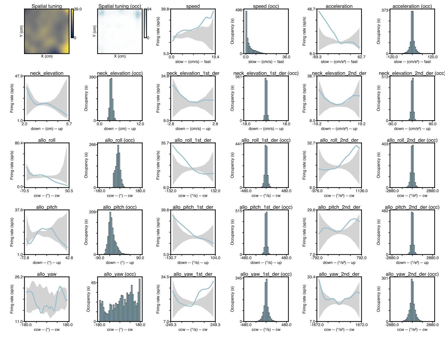
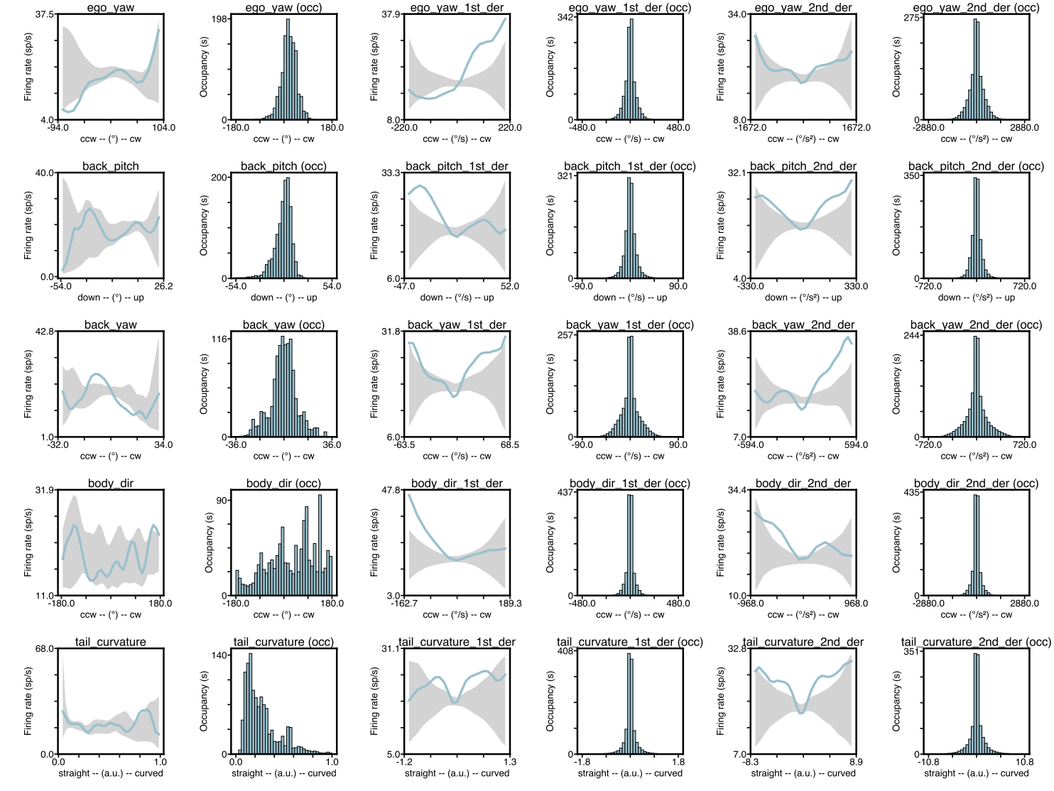
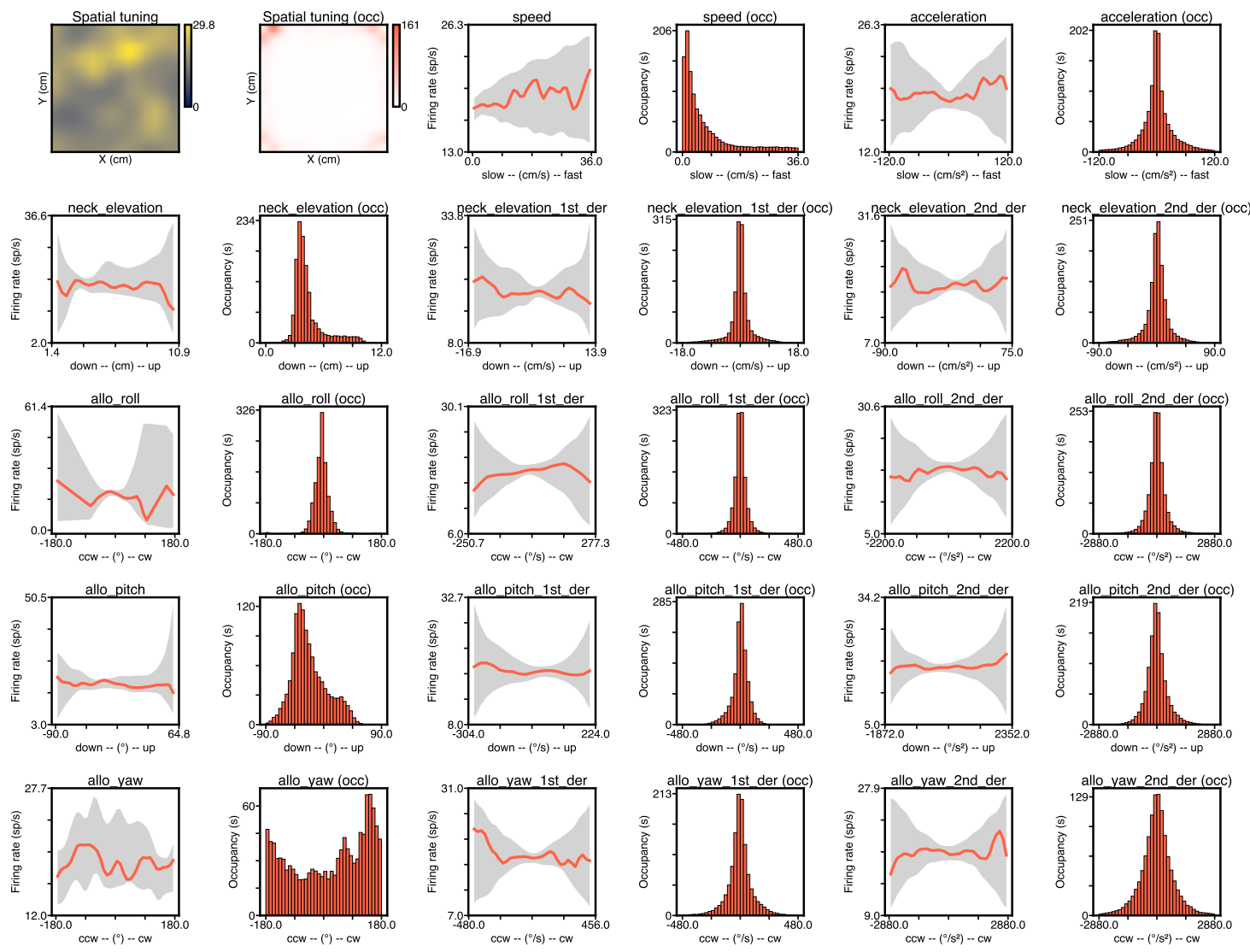
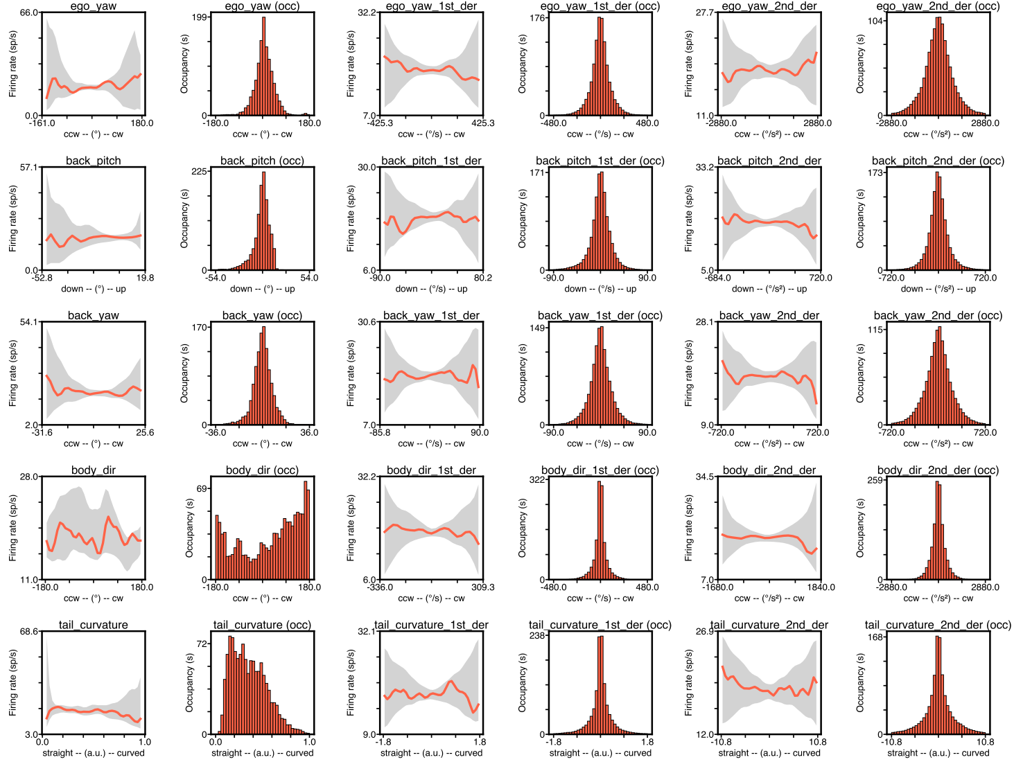
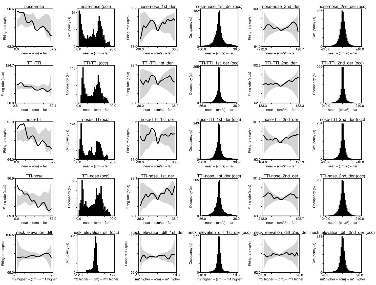
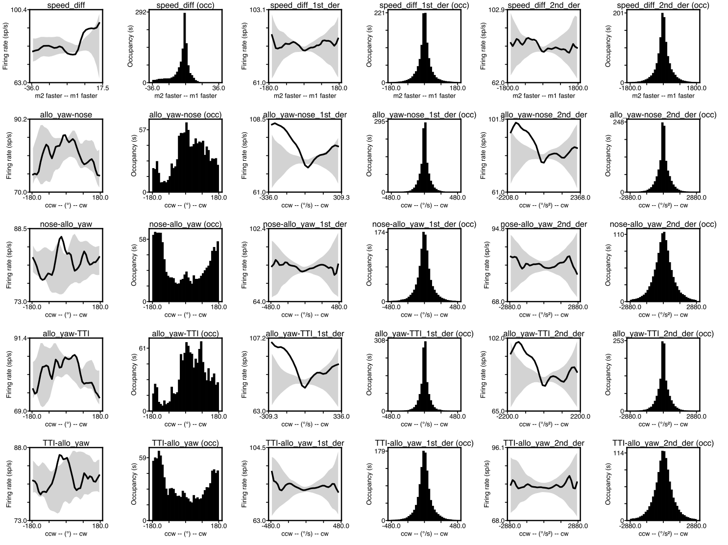
Once the Compute neuronal tuning curves function from the Analyze section has completed, you have the ability to plot its results. Output is one combined multi-page document per cluster: a behavioral page per temporal offset and per plot-feature group (individual.<mouse> and social) followed by the vocal pages — Page 1 (bout raster + pooled pre-USV usv_peth on top, usv_property_tuning continuous-property grid below) and Page 2 (usv_category_tuning watersheds + usv_category_peth per-category PETH grid). 1D ratemaps are drawn as a line spanning the plot, colored by the per-mouse palette (or the social color for social features). The 99% CI of the shuffled distribution is shown as a shaded band around the line.
To obtain this visualization, list the root directories of interest, select Plot neuronal tuning figures in the GUI and click Next and then Visualize:
Running this function results in the population of the tuning_curves subdirectory with one combined output per cluster (PDF by default; configurable in the GUI / settings):
├── 20250430_145017
│   ├── audio
│   │   ...
│   ├── ephys
│   │   ├── tuning_curves
│   │   │   ├── imec0_cl0000_ch361_good_neuronal_tuning.pdf
│   │   │   ...
│   ├── sync
│   │   ...
│   └── video
│       ...
For non-PDF formats, each page is written to a separate file with a _p{N}_{label} suffix (e.g. ..._p1_behavioral_beh_offset=0s_individual.<mouse>.png, ..._p3_vocal_a_male.png). PDF emits a single multi-page file.
An example of such tuning curves for one particular unit is shown below:
The rendering-side knobs live in the project-wide figures block of /usv-playpen/_parameter_settings/visualizations_settings.json (compute-side knobs such as smoothing_sd and behavioral_min_occupancy_seconds live in analyses_settings.json under calculate_neuronal_tuning_curves — see the Analyze page):
save_directory : default output directory for figures that aren’t written next to their source data (e.g. cross-session anatomy plots). Per-figure code may override this with an explicit
out_dirargument; per-cluster ratemaps and other session-bound figures always stay next to the data.fig_format : default output file format. For the per-cluster ratemap PDFs,
pdfproduces a single multi-page document;png/jpg/svgwrite one file per page.dpi : default raster resolution applied to every
fig.savefigcallsite that goes throughvisualizations.figure_io.save_figure.timestamp_in_name : when
true,_YYYYMMDD_HHMMSSis appended to figure stems by default. Session-bound figures opt out of this withtimestamp_in_name=falsesince their filenames already embed a session id or unit id.cmap : default matplotlib colormap used by every heatmap / ratemap callsite (one of
viridis,cividis,plasma,inferno,magma).make_behavioral_videoskeeps its owngeneral_figure_specs.cmapargument and is unaffected.
"figures": {
    "save_directory": "/mnt/falkner/Bartul/figures",
    "fig_format": "svg",
    "dpi": 300,
    "timestamp_in_name": true,
    "cmap": "inferno"
}
Visualize 3D behavior (figure/video)
Once 3D tracked data is available, you can visualize animal social behavior, either in figure or video. This GUI segment allows for a wide array of options in creating such visualizations. For example, you can choose whether you want to view the interaction from above or the side, and you can also choose to rotate the view as the behavior unfolds.
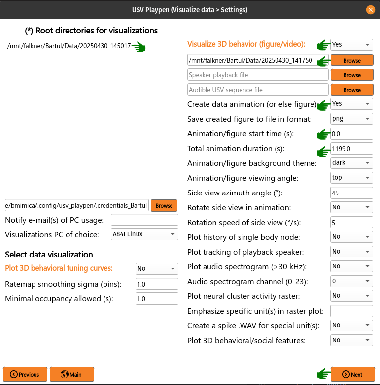
To obtain this visualization, you need to list the root directories of interest (it is best to stick with one), select the Visualize 3D behavior (figure/video) option in the GUI, insert the arena directory for that session, pick all desired figure features, click Next and then Visualize. It is important to point out that there are many more features available in the visualization_settings.json file than are available in the GUI, and these options are explained in detail several sections below:
Running this function results in the creation of the data_animation_examples subdirectory (if it has not been created already), and the figure/video will be saved inside:
├── 20250430_145017
│   ├── audio
│   │   ...
│   ├── data_animation_examples
│   │   ├── 20250430_145017_3D_30045fr_dark_topview_Bartul.png
│   │   ├── 20250430_145017_3D_30045-30795fr_dark_topview_Bartul.mp4
│   │   ...
│   ├── ephys
│   │   ...
│   ├── sync
│   │   ...
│   └── video
│       ...
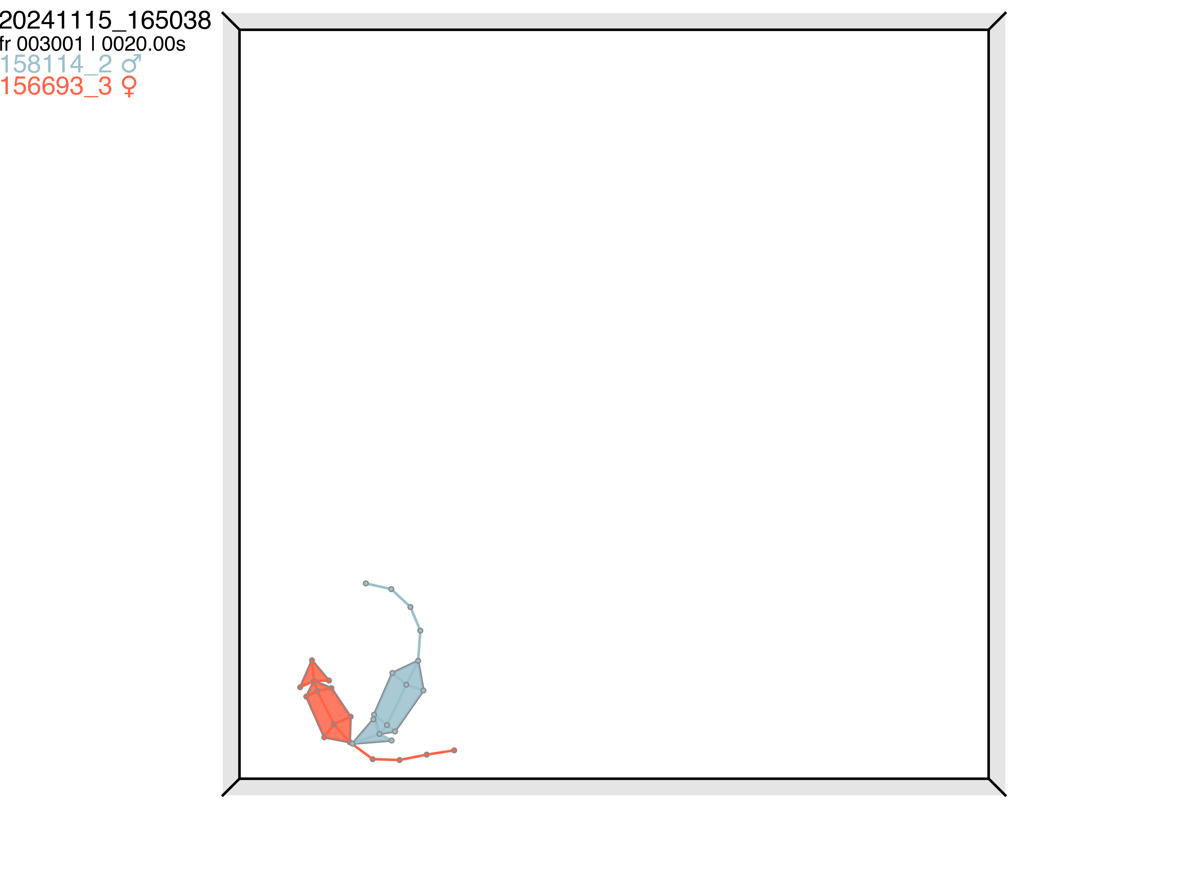
An example figure of male-female courtship behavior (as visualized from the top view with a light background) is shown below:
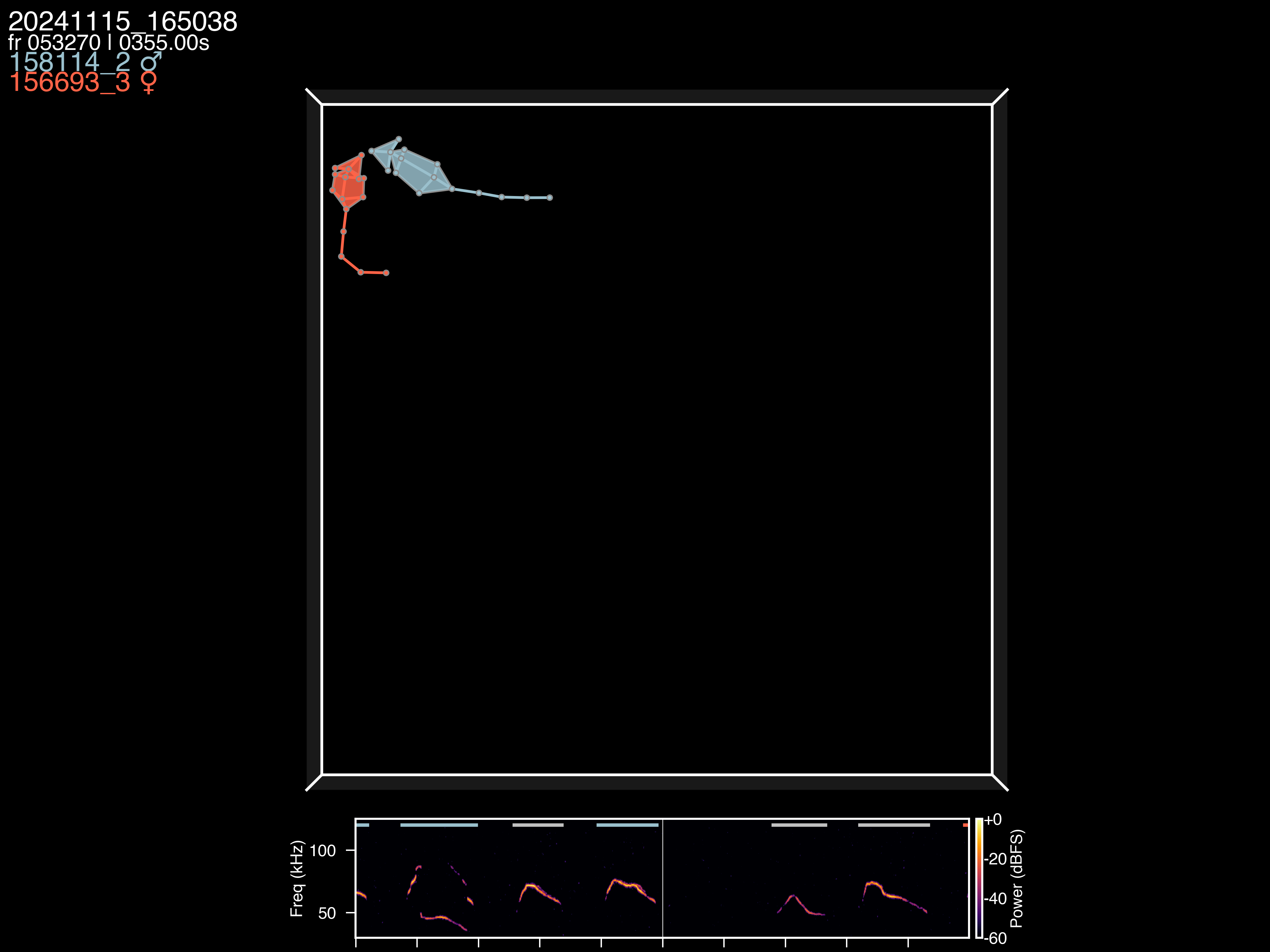
Another example male-female courtship interaction with a live spectrogram subplot, with vocalizations labeled by color of animal they were assigned to:
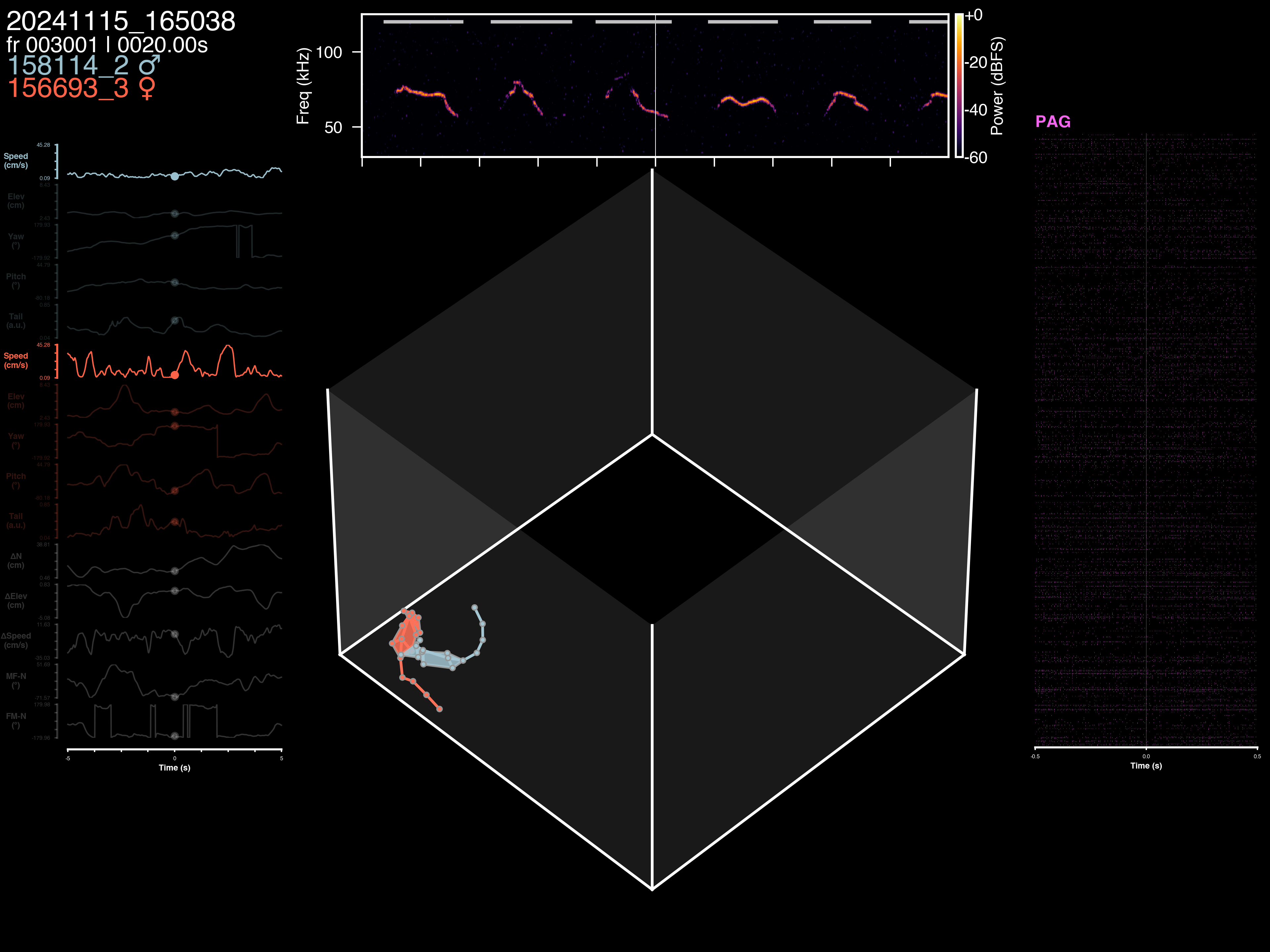
An example side view of a male-female courtship interaction with spectrogram, raster plot and behavioral features subplots:
An example of an animated male-female courtship interaction with a light background, side view and history of both animals’ heads:
An example of an animated male-female courtship interaction with a dark background, top view and spectrogram with assigned vocalizations:
The /usv-playpen/_parameter_settings/visualization_settings.json file contains a section only partially modifiable in the GUI, but it can entirely be modified manually in the visualization_settings.json file:
arena_directory : path to the directory with the 3D tracked arena data
speaker_audio_file : path to the audio file containing the playback speaker sound
sequence_audio_file : path to the frequency-shifted audio file containing the audible vocalizations
animate_bool : boolean value indicating whether to animate the figure or not (“No” creates figure)
video_start_time : start time of the figure/video in seconds
video_duration : duration of the video in seconds
plot_theme : “dark” or “light” plot background
save_fig : if True, the figure will be saved in the data_animation_examples subdirectory
view_angle : “top” or “side” view of social behavior in the playpen arena
side_azimuth_start : azimuth angle of the side view (in deg)
rotate_side_view_bool : rotate the side view or not (NB: angles wrap around)
rotation_speed : rotation speed of the side view (in deg/s)
history_bool : plot the location history of one body node
speaker_bool : plot the playback speaker
spectrogram_bool : plot the spectrogram of the audio segment
spectrogram_ch : channel of the audio segment to plot
raster_plot_bool : plot the live spiking raster of the neural data
raster_selection_criteria : criteria for selecting the neurons to plot in the raster
raster_selection_criteria (brain_areas) : list of brain areas to include in the raster plot
raster_selection_criteria (other) : list of other criteria to include in the raster plot (e.g., “good” for unit type)
raster_special_units : unit(s) to highlight in the raster plot (e.g., “imec0_cl0000_ch361”)
spike_sound_bool : make spike sound each time the highlighted unit spikes
beh_features_bool : plot the behavioral features dynamics subplot
beh_features_to_plot : list of behavioral features in the subplot
special_beh_features : list of highlighted behavioral features in the subplot
Parameters specific to the arena figure include:
arena_node_connections_bool : plots connections between corner and nearest microphones
arena_axes_lw : line width of the arena axes
arena_mics_lw : line width of the microphones
arena_mics_opacity : opacity of the microphones
plot_corners_bool : plot different color spheres in corners of the arena
corner_size : size of the corner spheres
corner_opacity : opacity of the corner spheres
plot_mesh_walls_bool : plot the mesh walls of the arena
mesh_opacity : opacity of the mesh walls
active_mic_bool : plots the active microphone (whose spectrogram is shown)
inactive_mic_bool : plots the inactive microphones (whose spectrograms are not shown)
inactive_mic_color : color of the inactive microphones
text_fontsize : font size of the text in the arena figure
speaker_opacity : opacity of the playback speaker
Parameters specific to the mouse figure include:
node_bool : plot mouse body nodes as spheres
node_size : size of the body node spheres
node_opacity : opacity of the body node spheres
node_lw : line width of the body node spheres
node_connection_lw : plots connections between body nodes
body_opacity : opacity of the body polygons connected with nodes
history_point : plot history of particular body point
history_span_sec : time span of the history in seconds (will fail if history is set to start before tracking!)
history_ls : line style of the history plot (e.g., “-”, “–”, “-.”, “:”)
history_lw : line width of the history plot
Parameters specific to subplots include:
beh_features_window_size : time window of the behavioral features subplot (in s, will fail if is set beyond tracking boundaries!)
raster_window_size : time window of the raster subplot (in s, will fail if is set beyond tracking boundaries!)
raster_lw : horizontal line width of spikes in the raster plot
raster_ll : vertical line length of spikes in the raster plot
spectrogram_cbar_bool : plot spectrogram colorbar
spectrogram_plot_window_size : time window of the spectrogram subplot (in s, will fail if is set beyond tracking boundaries!)
spectrogram_power_limit : lower and upper limits of the spectrogram colorbar (in dB)
spectrogram_frequency_limit : lower and upper limits of the spectrogram frequency axis (in Hz)
spectrogram_yticks : y-axis ticks of the spectrogram (in Hz)
spectrogram_stft_nfft : window size for the spectrogram calculation
plot_usv_segments_bool : plot the DAS-detected USV segments in the spectrogram
usv_segments_ypos : y-axis position of the USV segments in the spectrogram (in Hz)
usv_segments_lw : line width of the USV segments in the spectrogram
"make_behavioral_videos": {
    "arena_directory": "",
    "speaker_audio_file": "",
    "sequence_audio_file": "",
    "animate_bool": false,
    "video_start_time": 567.19,
    "video_duration": 5.0,
    "plot_theme": "dark",
    "save_fig": true,
    "view_angle": "top",
    "side_azimuth_start": 45,
    "rotate_side_view_bool": false,
    "rotation_speed": 5,
    "history_bool": false,
    "speaker_bool": false,
    "spectrogram_bool": false,
    "spectrogram_ch": 0,
    "raster_plot_bool": false,
    "raster_selection_criteria": {
      "brain_areas": [],
      "other": [
        "good"
      ]
    },
    "raster_special_units": [
      ""
    ],
    "spike_sound_bool": false,
    "beh_features_bool": false,
    "beh_features_to_plot": [],
    "special_beh_features": [],
    "general_figure_specs": {
      "fig_format": "png",
      "fig_dpi": 600,
      "animation_codec": "h264_nvenc",
      "animation_codec_preset_flag": "p5",
      "animation_codec_tune_flag": "hq",
      "animation_writer": "ffmpeg",
      "animation_format": "mp4"
    },
    "arena_figure_specs": {
      "arena_node_connections_bool": false,
      "arena_axes_lw": 1.0,
      "arena_mics_lw": 0.75,
      "arena_mics_opacity": 0.25,
      "plot_corners_bool": false,
      "corner_size": 1.0,
      "corner_opacity": 1.0,
      "plot_mesh_walls_bool": true,
      "mesh_opacity": 0.1,
      "active_mic_bool": false,
      "inactive_mic_bool": true,
      "inactive_mic_color": "#898989",
      "text_fontsize": 10,
      "speaker_opacity": 1.0
    },
    "mouse_figure_specs": {
      "node_bool": true,
      "node_size": 3.5,
      "node_opacity": 1.0,
      "node_lw": 0.5,
      "node_connection_lw": 1.0,
      "body_opacity": 0.85,
      "history_point": "Head",
      "history_span_sec": 5,
      "history_ls": "-",
      "history_lw": 0.75
    },
    "subplot_specs": {
      "beh_features_window_size": 10,
      "raster_window_size": 1,
      "raster_lw": 0.1,
      "raster_ll": 0.9,
      "spectrogram_cbar_bool": true,
      "spectrogram_plot_window_size": 1,
      "spectrogram_power_limit": [
        -60,
        0
      ],
      "spectrogram_frequency_limit": [
        30000,
        125000
      ],
      "spectrogram_yticks": [
        50000,
        100000
      ],
      "spectrogram_stft_nfft": 512,
      "plot_usv_segments_bool": true,
      "usv_segments_ypos": 120000,
      "usv_segments_lw": 1.25
    }
}