Analyze

This page explains how to use the data analyses functionalities in the usv-playpen GUI.

In order to run any of the functions detailed below, select an experimenter name from the dropdown menu and click the Analyze button on the GUI main display:

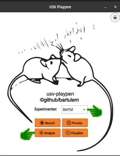
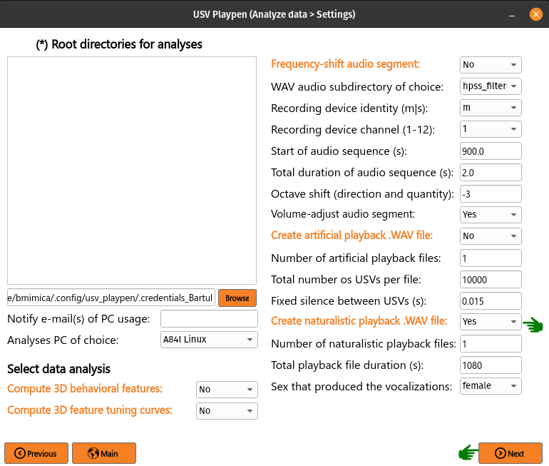
Clicking the Analyze button will open a new window with all the offered functionalities (see below):

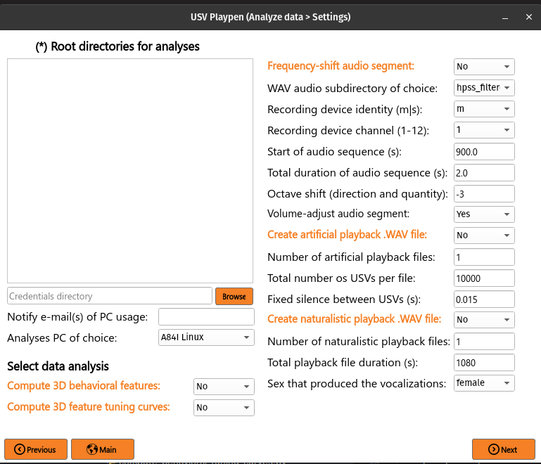
All the main functions are outlined in orange, and black fields are function-specific options tunable by the user in the GUI. It is important to note that these are not necessarily all the options the user can set, and the full list of options can be found under each function in the /usv-playpen/_parameter_settings/analyses_settings.json file. Each time the user clicks the Next button in the window above, analyses_settings.json is modified to the newest input configuration.

The Root directories field enables you to list the directories containing the data you want to analyze. Each root directory should be in its own row; for example, three sessions should be listed as follows:

/mnt/falkner/Bartul/20250430_145017
/mnt/falkner/Bartul/20250430_165730
/mnt/falkner/Bartul/20250430_182145

Compute 3D behavioral features

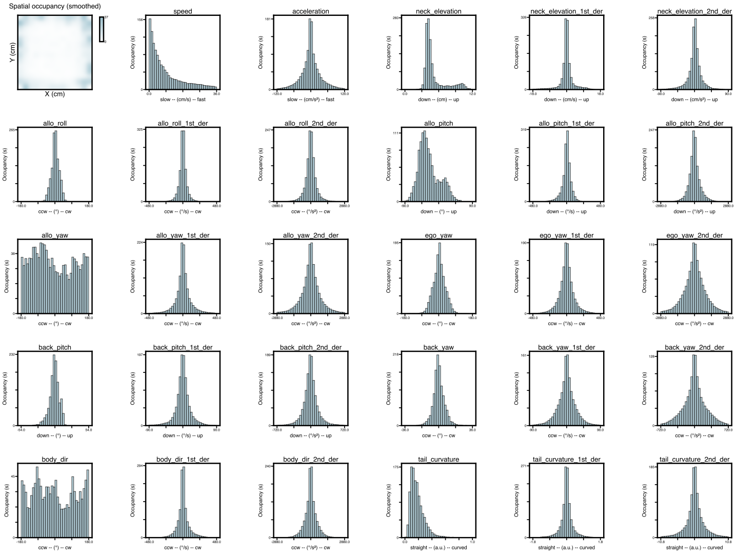
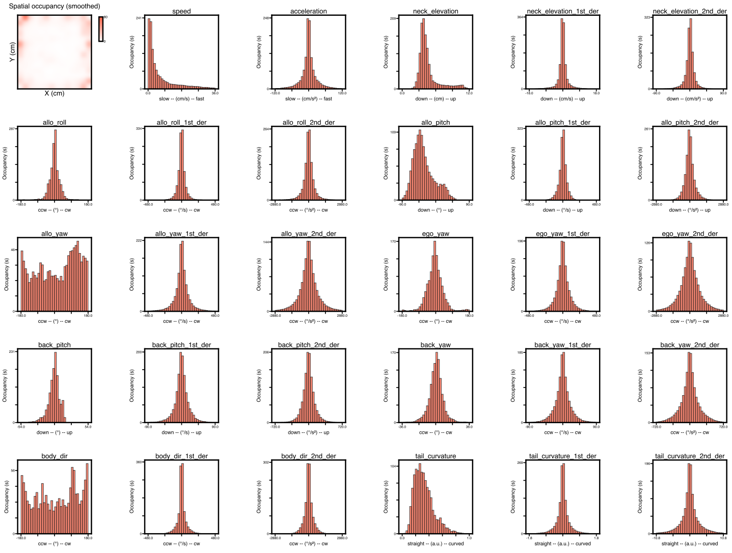
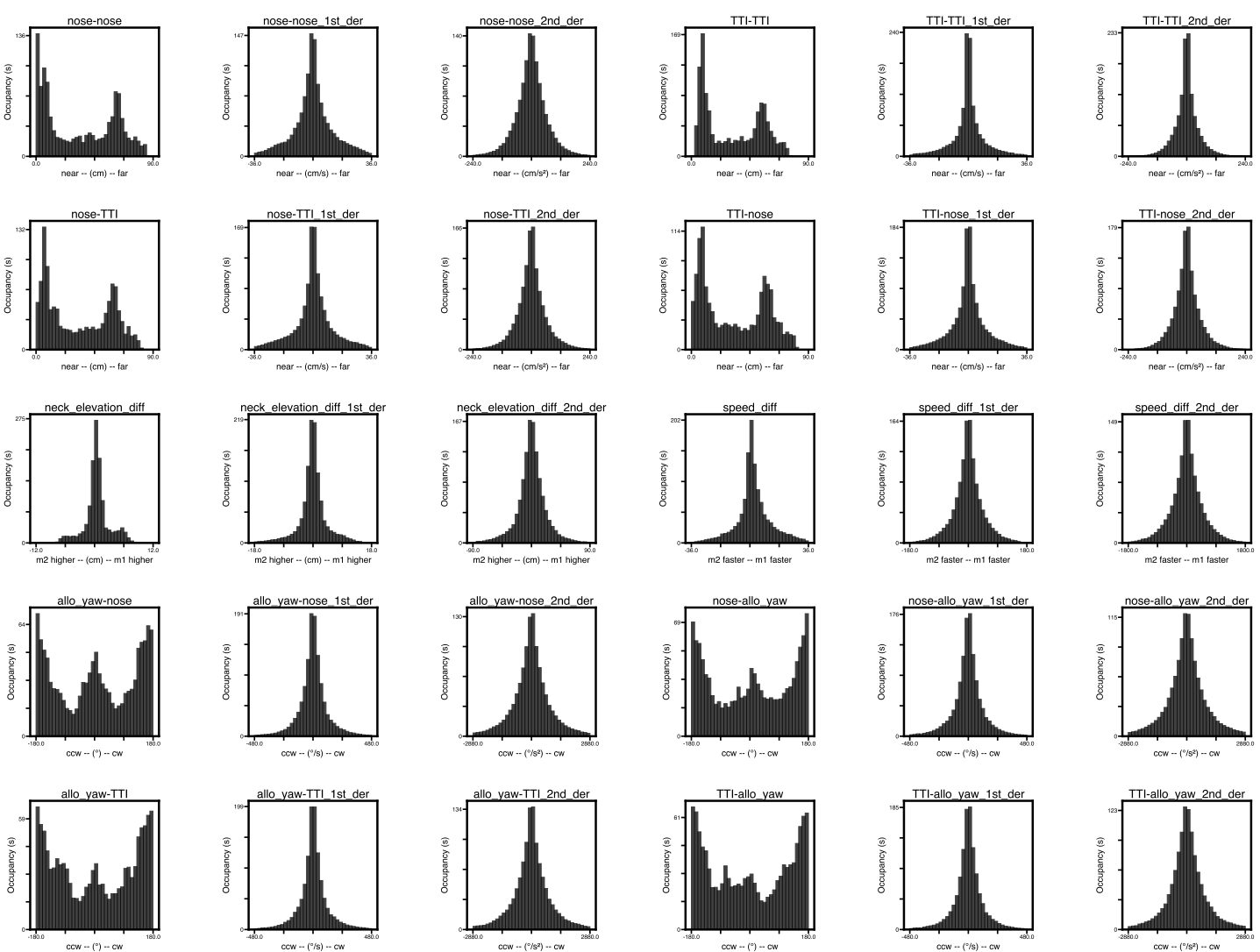
Once 3D tracking data is available, you can compute behavioral features. These can be individual features specific to each mouse (i.e., spatial location, speed, posture, etc.) or social features (assuming two or more mice) that describe the relationship between the mice (i.e., distance, angle, etc.). The output of this analysis are two files: [1] CSV file containing each measured feature in each column, and [2] a PDF file containing graphs for the observed distribution of each feature. To run this analysis in the GUI, you need to list the root directories of interest, select Compute 3D behavioral features, click Next and then Analyze:

The analysis results in the creation of [1] a CSV file containing behavioral features, [2] a PDF file showing occupancy distributions for each feature, and both can be found as shown below:

├── 20250430_145017
│   ├── audio
│   │   ...
│   ├── ephys
│   │   ...
│   ├── sync
│   │   ...
│   │
│   └── video
│       ├── 20250430_145027.21241563
│       ...
│       ├── 20250430145035_camera_frame_count_dict.json
│       ├── 20250430145035
│       │    ├── 20250430145035_points3d_translated_rotated_metric_behavioral_features.csv
│       │    ├── 20250430145035_points3d_translated_rotated_metric_behavioral_features_histograms.pdf
│       ...

The behavioral_features.csv file should look similar to an example table below:

┌─────────────────┬─────────────────┬─────────────────┬────────────────┬───┬
│ 158114_2.spaceX ┆ 158114_2.spaceY ┆ 158114_2.spaceZ ┆ 158114_2.speed ┆ … ┆
│ ---             ┆ ---             ┆ ---             ┆ ---            ┆   ┆
│ f64             ┆ f64             ┆ f64             ┆ f64            ┆   ┆
╞═════════════════╪═════════════════╪═════════════════╪════════════════╪═══╪
│ -26.841561      ┆ -23.796571      ┆ 2.922045        ┆ NaN            ┆ … ┆
│ -26.844099      ┆ -23.798917      ┆ 2.923149        ┆ 0.426783       ┆ … ┆
│ -26.848196      ┆ -23.802833      ┆ 2.925208        ┆ 0.505712       ┆ … ┆
│ -26.85301       ┆ -23.807948      ┆ 2.927885        ┆ 0.598469       ┆ … ┆
│ -26.859138      ┆ -23.813435      ┆ 2.930909        ┆ 0.692332       ┆ … ┆
│ …               ┆ …               ┆ …               ┆ …              ┆ … ┆
│ -4.515579       ┆ -28.340828      ┆ 3.667301        ┆ 11.337689      ┆ … ┆
│ -4.583698       ┆ -28.336554      ┆ 3.668319        ┆ 9.594388       ┆ … ┆
│ -4.638644       ┆ -28.332085      ┆ 3.668867        ┆ 7.809649       ┆ … ┆
│ -4.678483       ┆ -28.327466      ┆ 3.668817        ┆ 6.153409       ┆ … ┆
│ -4.699602       ┆ -28.324635      ┆ 3.668698        ┆ 4.805457       ┆ … ┆
└─────────────────┴─────────────────┴─────────────────┴────────────────┴───┴

An example of typical individual and social feature distributions is shown below:

The /usv-playpen/_parameter_settings/analyses_settings.json file contains a section not modifiable in the GUI itself, but it can be modified manually:

head_points : head skeleton node names (order matters!)
tail_points : tail skeleton node names (order matters!)
back_root_points : back skeleton node names (order matters!)
derivative_bins : number of bins to compute derivatives over

  "compute_behavioral_features": {
      "head_points": [
        "Head",
        "Ear_R",
        "Ear_L",
        "Nose"
      ],
      "tail_points": [
        "TTI",
        "Tail_0",
        "Tail_1",
        "Tail_2",
        "TailTip"
      ],
      "back_root_points": [
        "Neck",
        "Trunk",
        "TTI"
      ],
      "derivative_bins": 10
}

Compute neuronal tuning curves

Having recorded unit activity, social behavior, and ultrasonic vocalizations (USVs), you might be interested whether individual units encode specific behavioral features and / or vocal properties. To get at this, you can compute session-averaged tuning curves capturing the relationship between the firing rate of each unit and (a) each 3D behavioral feature, and (b) USV-anchored quantities — a pooled pre-USV PETH (usv_peth), within-USV firing rate as a function of each continuous acoustic property (usv_property_tuning over duration, mean / peak frequency, bandwidth, amplitude, spectral entropy, mask number), within-USV firing rate as a function of categorical USV labels (usv_category_tuning over VAE / QLVM category and supercategory), and a per-category time-resolved peri-USV PETH (usv_category_peth). Behavioral and vocal payloads are produced together and serialized into a single per-cluster pickle. To trigger this in the GUI, list the root directories of interest, select Compute neuronal tuning curves, click Next and then Analyze (a progress bar will appear in the terminal while the analysis is running):

The analysis results in the creation of a tuning_curves subdirectory containing a pickle file for each recorded unit. Each pkl carries (when the corresponding inputs exist) beh_offset=*s blocks for behavioral tuning, plus usv_peth (PETH), usv_property_tuning (continuous property tuning), usv_category_tuning (categorical), usv_category_peth (per-category PETH), and behavioral_metadata / usv_metadata blocks describing the compute config:

├── 20250430_145017
│   ├── audio
│   │   ...
│   ├── ephys
│   │   ├── tuning_curves
│   │   │   ├── imec0_cl0000_ch361_good_tuning_curves_data.pkl
│   │   │   ...
│   ├── sync
│   │   ...
│   └── video
│       ...

The /usv-playpen/_parameter_settings/analyses_settings.json file contains a section only partially modifiable in the GUI, but it can be modified manually:

temporal_offsets : list of temporal offsets between spikes and behavior (in seconds, negative values: spikes precede behavior) for which the tuning curves will be calculated (adding values to the list increases the time needed for analysis drastically)
n_shuffles : number of spike train shuffles (increasing this number increases the time needed for analysis drastically)
shuffle_seed : base seed for the spike-train shuffle null distribution; fixing it makes the significance verdicts reproducible across runs
total_bin_num : total number of bins for a 1D behavioral / vocal-property feature
n_spatial_bins : number of spatial bins (2D behavioral feature)
spatial_scale_cm : maximum distance from center of arena to one edge (in cm)
shuffle_seconds_range : [min, max] of the uniform circular shift (in s) used to build the null distribution
peth_window_seconds : [start, stop] of the pre-USV PETH window (in s)
peth_bin_seconds : PETH bin width (in s)
bout_quiet_seconds : inter-bout silence required to define a new bout (in s)
vocal_require_clean_post_anchor : if true, the time after the USV onset must be free of contaminating USVs to keep the anchor
vocal_require_clean_prior_anchor : if true, the lookback window must also be free of contaminating USVs
n_usv_min_self : minimum self-side USV count for the self plots to be computed
n_usv_min_partner : minimum partner-side USV count for the partner plots to be computed
n_usv_min_category : minimum per-category USV count to retain that category in the categorical tuning layouts
behavioral_min_occupancy_seconds : minimum behavioral occupancy per bin (in s) to draw that bin in 1D feature plots; persisted into behavioral_metadata
usv_property_min_occupancy_seconds : minimum vocal-property occupancy per bin (in s) to keep the rate estimate finite
include_partner_vocalization_tuning_bool : also compute partner-side vocal tuning when its threshold is met
shuffle_chunk_size : how many shuffles to materialize at once (memory / speed knob)
smoothing_sd : standard deviation of the Gaussian kernel (in bins) applied to ratemaps and shuffle distributions; 0 disables smoothing
circular_features : list of behavioral feature suffixes that are wrap-around in nature (e.g. allo_yaw, body_dir); used by the triage helpers to detect divergence runs that span the bin-0 / bin-N boundary

"calculate_neuronal_tuning_curves": {
    "temporal_offsets": [0],
    "n_shuffles": 1000,
    "shuffle_seed": 0,
    "total_bin_num": 36,
    "n_spatial_bins": 196,
    "spatial_scale_cm": 32,
    "shuffle_seconds_range": [20, 60],
    "peth_window_seconds": [-2, 0],
    "peth_bin_seconds": 0.05,
    "bout_quiet_seconds": 2.0,
    "vocal_require_clean_post_anchor": true,
    "vocal_require_clean_prior_anchor": false,
    "n_usv_min_self": 100,
    "n_usv_min_partner": 30,
    "n_usv_min_category": 20,
    "behavioral_min_occupancy_seconds": 1.0,
    "usv_property_min_occupancy_seconds": 0.25,
    "include_partner_vocalization_tuning_bool": false,
    "shuffle_chunk_size": 50,
    "smoothing_sd": 1.0,
    "circular_features": ["allo_yaw", "body_dir"]
}

Per-cluster `triage_stats` block

Each per-cluster pkl also carries a triage_stats block — a flat collection of pre-computed scalar summaries that the downstream unit-triage aggregator consumes without re-touching spike or USV data. The keys mirror the per-modality structure of the rate payload:

vmi[emitter] — Vocalization Modulation Index (Mimica et al.). For each emitter side: vmi in [-1, 1], paired Wilcoxon wilcoxon_statistic / wilcoxon_pvalue over the per-bout (FR_baseline, FR_USV) pairs, plus n_bouts, fr_baseline_per_bout and fr_usv_per_bout arrays. VMI = (FR_USV − FR_baseline) / (FR_USV + FR_baseline), where FR_baseline is the mean firing rate in the bout_quiet_seconds-wide window before each bout and FR_USV is the mean over USVs in each bout of (spikes during USV) / (USV duration). Bouts whose baseline window starts before t = 0 are NaN-baselined.
usv_peth[emitter], usv_property_tuning[emitter][prop], usv_category_peth[emitter][cat_feat], behavioral[offset_key][feature_key] — per-direction (excitation / suppression) divergence-segment analysis with n_bins total above (or below) the shuffle band, max_run consecutive-bin run length, run_start_idx / run_end_idx (and the corresponding axis-value bounds), peak_idx / peak_z. For 1D feature axes also peak_abs_z, peak_signed_z, selectivity = (max−min)/(max+min), monotonicity (Spearman ρ between bin index and rate), and is_circular (behavioral only). The PETH variants additionally carry ramp_index (a two-point pre-USV shape descriptor).
usv_category_tuning[emitter][cat_feat] — categorical (no run analysis): peak_abs_z, best_cat, n_sig_categories (count of categories outside the [p0.5, p99.5] shuffle band), selectivity.
spatial[offset_key][feature_key] — 2D place-cell diagnostics: info_rate_bps (Skaggs information rate), sparsity, coherence (Pearson correlation between each bin and the mean of its 8 neighbors), plus the unshuffled peak rate and its grid coordinates. The 2D spatial map is computed without shuffles, so peak Z is not defined; this block reports the rate / occupancy diagnostics instead.

Cross-session unit-triage aggregator

Once Compute neuronal tuning curves has produced per-cluster pkls across many sessions, the analyses_notebooks/neuronal_tuning_summary.ipynb notebook drives aggregate_units_across_conditions: for each condition (one .txt session list per condition), every session’s pkls are loaded, the same significance rules applied to the pre-computed triage_stats, and the results joined with unit_catalog.csv to enrich each cluster with mouse_id, rec_date, and brain_area. Same-day duplicate units (one physical unit across replicate sessions) are collapsed into a single record with per-session evidence stacked underneath each modality. This step never re-loads spike or USV data — it is a pure pkl-to-pickle pass — so thresholds can be swept without re-running compute.

The output is a single pickle <out_dir>/unit_triage_<YYYYMMDD>_<HHMMSS>.pkl with:

thresholds_used — the threshold values that produced this run.
conditions_included / sessions_skipped — what made it in, what was missing.
n_units_total / n_units_per_condition — bookkeeping counts.
units — keyed by unit_uid = f"{mouse_id}_{rec_date}_{unit_id}", each carrying identity, anatomy_region, and a conditions block. For every condition, every modality reports n_significant / n_tested / consistency plus a per_session list of evidence rows and an aggregate scalar.

The /usv-playpen/_parameter_settings/analyses_settings.json file holds the gate thresholds in a dedicated section:

z_threshold : magnitude threshold on per-direction peak_z. Used for usv_peth, usv_property_tuning, usv_category_peth, usv_category_tuning (peak Z gate), and behavioral modalities.
min_consecutive_bins : minimum consecutive-bin run length to flag a direction (excit or suppress). Combined with the z_threshold gate; does not apply to usv_category_tuning (no axis order) or spatial (uses Skaggs info instead).
vmi_alpha : two-sided Wilcoxon p-value threshold for VMI significance.
vmi_min_bouts : minimum bout count required to consider VMI meaningful.
spatial_info_bps_threshold : Skaggs information-rate threshold (bits/spike) for the spatial flag.

"detect_interesting_tuning_neurons": {
    "z_threshold": 3.0,
    "min_consecutive_bins": 3,
    "vmi_alpha": 0.01,
    "vmi_min_bouts": 10,
    "spatial_info_bps_threshold": 0.5
}

The notebook is a thin wrapper: edit CONDITION_TO_SESSION_LIST to point at the .txt lists, optionally adjust THRESHOLDS, and run all cells. The pickle it produces is the input to all downstream cross-session plotting.

Compute inter-vocalization-interval (inter-USV interval) distributions

This analysis pools same-emitter inter-vocalization intervals (inter-USV intervals) across one or more cohorts and (optionally) sweeps a 1D Gaussian Mixture Model (GMM) on the log-transformed inter-USV intervals to identify behavioral regimes (e.g. “short” intra-bout intervals vs “long” inter-bout intervals). Unlike the other analyses on this page, this one is not driven by the Root directories GUI field — it is driven by one or more session-list text files, each containing one session root per line. This lets multi-cohort comparisons be assembled by simply pointing at additional list files (each session is tagged with the list file it came from for downstream grouping).

By convention, track_names[0] in each session’s tracking H5 is treated as the male and track_names[1] as the female. Each session-list path and each line within is run through configure_path so paths written for Linux/Mac/Windows resolve correctly on the host platform.

Both interval definitions are computed on every run (no flag, no toggle):

s2s : start[i+1] - start[i] (literature standard)
e2s : start[i+1] - stop[i] (alternate; can be negative for overlapping calls and is dropped via the > 0 filter, with the dropped count reported per session per mode)

Both definitions share the same per-session pass over the noise-filtered USV table, so emitting both costs essentially the same as emitting one and lets downstream code compare them (e.g. quantify how much overlap the e2s filter introduces) without re-running the analysis.

Each run produces a single self-describing HDF5 archive in output_directory:

/path/to/output_directory
└── usv_interval_analysis_<YYYYMMDD>_<HHMMSS>.h5

The archive’s structure (see usv_playpen.analyses.usv_interval_archive for the full schema):

Root /attrs – every JSON parameter that drove the run, plus created_at_iso, git_sha, source_lists and n_sessions_loaded, so a months-later reader is fully self-describing.
/<mode>/intervals – tidy one-row-per-inter-USV interval table (session_id, source_list, interval_type, sex, interval_s, log_interval, male_id, female_id).
/<mode>/drop_counts – per-sex count of dropped non-positive intervals (only meaningful for e2s).
/<mode>/gmm_fits (when fit_gmm is true) – the full GMM / t-mixture sweep with all four ICs (bic, aic, icl, cv_neg_loglik) and per-component parameters (logmean_k, logsd_k, weight_k, nu_k) per (sex, n_comp, rep) row. This table doubles as the model-parameter store; downstream plot helpers pick the best-rep row to rebuild the fitted mixture without refitting.
/<mode>/bootstrap_lrt – per-pair LRT summary with columns [sex, K_null, K_alt, lr_obs, null_mean, null_p95, null_max, p_value, B, n_subsample, model_class, alpha_used, K_selected_step_up]. K_selected_step_up is constant within each sex and records the per-sex K chosen by the step-up rule.
/<mode>/bootstrap_lrt_null – long-form bootstrap LR null draws, one row per (sex, K_null, K_alt, b) with the bootstrap statistic lr_b. Used to re-render the null-distribution panel without re-running the test.
/<mode>/attrs – alpha_effective (post-Bonferroni alpha if requested) plus the per-sex step-up-selected K (K_selected_male, K_selected_female).

The accompanying notebook (analyses_notebooks/usv_interval_mixture_models_plots.ipynb) reads the archive via the ivs.load_*_from_h5 helpers and renders the bootstrap LRT null-distribution panel (with broken-axis support when LR_obs falls far above the null), the BIC and AIC sweeps with the LRT-selected K highlighted, the best-fit mixture with per-component triangles labelled by bold (a), (b), … markers, a left-aligned text legend mapping each letter to its component median in seconds, an optional per-component pdf overlay, and a log-log Q-Q diagnostic embedded as an inset.

The /usv-playpen/_parameter_settings/analyses_settings.json file contains a section that should be modified manually (the GUI does not currently expose this analysis):

session_lists : list of paths to session-list text files (each line is one session root). The inter-USV interval notebook reads this list directly from JSON; do not duplicate paths in the notebook.
output_directory : directory in which to write the consolidated usv_interval_analysis_<YYYYMMDD>_<HHMMSS>.h5 archive (and where the notebook’s find_latest_archive looks)
noise_col_id : name of the noise classification column in the USV summary CSV
noise_categories : integer label(s) in noise_col_id that mark a USV as noise
fit_gmm : whether to run the GMM sweep after inter-USV interval extraction
n_components_min / n_components_max : range of mixture sizes to sweep
n_repeats : number of EM-init repeats per (key, n_components)
max_modes_reported : maximum number of mixture modes recorded per fit
random_seed_base : base seed; rep r uses random_seed_base + r
cv_n_folds : Number of K-fold splits for cross-validated log-likelihood. Defaults to 5. KFold uses shuffle=True for partition independence.
cv_n_init : Number of EM restarts inside each fold’s GMM fit during cross-validation. Defaults to 5 (smaller than the in-sample gmm_n_init because folds already average out EM noise).
gmm_n_init : Number of EM restarts per in-sample GMM fit. Defaults to 10. Higher values make EM more robust to local optima but cost compute.
gmm_reg_covar : Regularisation added to component covariances (sklearn’s reg_covar). Defaults to 1e-4 (above the sklearn default of 1e-6) to prevent small components from collapsing to near-singular covariances on log-inter-USV interval data.
tau : Posterior threshold for the LEFT component when computing inter-component decision boundaries. 0.5 gives the standard Bayes boundary. Higher values move the boundary toward the left component, making the “short” regime more conservative.
figures_directory : Directory in which the inter-USV interval notebook saves rendered figures. Run through configure_path so a Linux-style path resolves on Mac / Windows hosts.
bins_per_sex : Object mapping "male" and "female" to integer histogram bin counts for the fit-plot panels. Females typically have far fewer samples and benefit from fewer bins (e.g. 30) so the histogram isn’t fragmented into spurious troughs and peaks.
plot_log_xlims : Two-element list [low, high] (in log-seconds) clipping the x-axis of every inter-USV interval plot. Defaults to [-5.0, 5.0] (~6.7 ms to ~148 s).
model_class : Mixture model class. One of:
- "t" (default): Student-t mixture in log-space. One heavy-tailed t-component absorbs the long-pause tail, freeing the remaining components to track only the main-peak structure. Recommended for inter-USV interval bout-structure analysis. Per-component degrees of freedom (nu) are estimated jointly with the location and scale via the Peel & McLachlan (2000) EM algorithm.
- "gauss": log-Gaussian mixture (the original implementation, kept for back-compatibility). With heavy-tailed inter-USV interval distributions this typically requires several wide Gaussians to model the long pause tail, inflating the apparent component count. Use only when you specifically want the classical log-normal mixture.
Both classes share the same IC sweep (BIC / AIC / ICL / CV-LL) and selection rules; the gmm_fits table inside the HDF5 archive gains a model_class column tagging which class produced each row, so artifacts from either class remain interpretable.
bootstrap_lrt_B : Number of parametric bootstrap replicates per pairwise LRT (McLachlan 1987; McLachlan & Peel 2000 Ch. 6). Defaults to 1000 (smooth null distribution + meaningful 99th-percentile reference line); reduce to 100-200 only for fast-iteration debugging.
bootstrap_lrt_n_subsample : Subsample size used for both observed and bootstrap fits, so the LR statistic is on the same N scale across them. Defaults to 15000. The test is asymptotically valid for any sufficiently large value; smaller subsamples trade some power for a faster run.
bootstrap_lrt_alpha : Significance threshold for the step-up rule. Defaults to 0.05.
bootstrap_lrt_bonferroni : If true, the per-pair alpha is divided by the number of consecutive K-pairs tested before applying the step-up rule. Defaults to false.

"compute_inter_usv_interval_distributions": {
    "session_lists": [
      "/mnt/falkner/Bartul/modeling/input_files/courtship_behavioral_intact_partners_sessions_list.txt"
    ],
    "output_directory": "/mnt/falkner/Bartul/modeling/usv_interval_results",
    "noise_col_id": "usv_supercategory",
    "noise_categories": [0],
    "fit_gmm": true,
    "n_components_min": 2,
    "n_components_max": 5,
    "n_repeats": 100,
    "max_modes_reported": 3,
    "random_seed_base": 0,
    "cv_n_folds": 5,
    "cv_n_init": 5,
    "gmm_n_init": 10,
    "gmm_reg_covar": 1e-4,
    "tau": 0.5,
    "figures_directory": "/mnt/falkner/Bartul/figures",
    "bins_per_sex": {"male": 80, "female": 30},
    "plot_log_xlims": [-5.0, 5.0],
    "model_class": "t",
    "bootstrap_lrt_B": 1000,
    "bootstrap_lrt_n_subsample": 15000,
    "bootstrap_lrt_alpha": 0.05,
    "bootstrap_lrt_bonferroni": false
}

Frequency shift audio segment

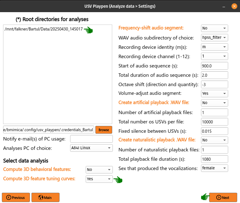
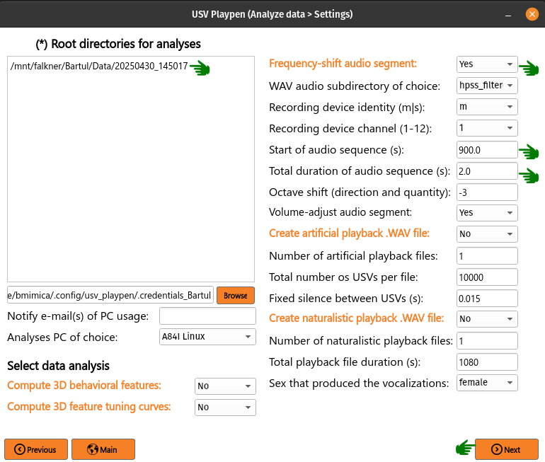
For presentation purposes, one might want to play audio data of mouse USVs. Since these are beyond human audible range, the only way is to frequency-shift them several octaves down. To achieve this in the GUI, you need to list the root directories of interest, select Frequency shift audio segment, choose the start time and duration of the segment, click Next and then Analyze:

The analysis results in the creation of a frequency_shifted_audio_segments subdirectory (if it is not already there) and a wave file in it containing the frequency-shifted segment:

├── 20250430_145017
│   ├── audio
│   │   ├── frequency_shifted_audio_segments
│   │   │   ├── m_20250430145035_ch01_cropped_to_video_hpss_filtered.wav_start=900.0s_duration=2.0s_octave_shift=-3_audible_denoised_tempo_adjusted.wav
│   ├── ephys
│   │   ...
│   ├── sync
│   │   ...
│   └── video
│       ...

Below you can find an example of a brief sequence of frequency-shifted mouse vocalizations:

The /usv-playpen/_parameter_settings/analyses_settings.json file contains a section only partially modifiable in the GUI, but it can be modified manually:

fs_audio_dir : audio subdirectory where the audio files are stored
fs_device_id : USGH device ID (e.g. “m” for main, “s” for secondary)
fs_channel_id : microphone channel ID (1-12)
fs_wav_sampling_rate : sampling rate of the audio devices in kHz
fs_sequence_start : start time of the audio segment in seconds
fs_sequence_duration : duration of the audio segment in seconds
fs_octave_shift : octave shift of the audio segment (e.g. -3 for 1/8 octave shift)
fs_volume_adjustment : whether to automatically increase the volume of the audio segment; recommended since the vocalizations are faint

"frequency_shift_audio_segment": {
    "fs_audio_dir": "hpss_filtered",
    "fs_device_id": "m",
    "fs_channel_id": 1,
    "fs_wav_sampling_rate": 250,
    "fs_sequence_start": 900.0,
    "fs_sequence_duration": 2.0,
    "fs_octave_shift": -3,
    "fs_volume_adjustment": true
}

Create artificial playback .WAV file

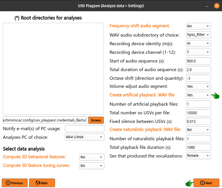
This function creates a .WAV file containing USV snippets. The snippets are randomly selected from the USV snippet repository in the specified directory and concatenated with inter-pulse intervals (IPIs) of a specified duration. The resulting .WAV file can be used for playback experiments. To achieve this in the GUI, select Create artificial playback .WAV file (no need to list root directories!), select total number of files to be created, number of vocalizations in each one, click Next and then Analyze:

The analysis results in the creation of three files: [1] WAV file containing playback vocalizations, [2] a spacing text file informing you of the duration of each vocalization in order, and [3] a usvids text file containing the identity of each vocalization snippet if you need to go back and look at what it was:

/mnt/falkner/Bartul/usv_playback_experiments/usv_playback_files
├── usv_playback_n=10000_20250506_190808.wav
├── usv_playback_n=10000_20250506_190808_spacing.txt
├── usv_playback_n=10000_20250506_190808_usvids.txt
...

The /usv-playpen/_parameter_settings/analyses_settings.json file contains a section only partially modifiable in the GUI, but it can be modified manually:

num_usv_files : number of artificial playback files to be created
total_usv_number : total number of USVs to be included in one playback file
ipi_duration : inter-pulse interval duration in seconds
wav_sampling_rate : sampling rate of the playback .WAV file in kHz
playback_snippets_dir : subdirectory where the USV snippets are stored
playback_seed : optional RNG seed for reproducible snippet selection and assembly; null draws a fresh random stimulus each run, an integer reproduces the same stimulus

"create_usv_playback_wav": {
    "num_usv_files": 1,
    "total_usv_number": 10000,
    "ipi_duration": 0.015,
    "wav_sampling_rate": 250,
    "playback_snippets_dir": "usv_playback_snippets_loudness_corrected",
    "playback_seed": null
}

Create naturalistic playback .WAV file

This function creates a .WAV file containing naturalistic sequences of USV snippets. The snippets are randomly selected from the female or male USV snippet repository in the specified directory and assembled into sequences with empirically derived inter-event intervals. The resulting .WAV file can be used for playback experiments. To achieve this in the GUI, select Create naturalistic playback .WAV file (no need to list root directories!), select total number of files to be created, number of vocalizations in each one, click Next and then Analyze:

Inter-USV intervals (IUIs) and inter-sequence intervals (ISIs) are sampled from a sex-specific 3-component Gaussian mixture model (GMM) fit to log-transformed empirical interval data. Sex is inferred automatically from the naturalistic_playback_snippets_dir_prefix setting (e.g. "female" or "male"). Specifically:

IUI is drawn from the first GMM component (shortest intervals, ~60 ms peak): exp(N(mean[0], sd[0]))
ISI is drawn from the third GMM component (longest intervals, seconds-scale): exp(N(mean[2], sd[2]))
Sequence length is drawn from N(13, 5) clipped to [3, 23] USVs

The analysis results in the creation of three files: [1] WAV file containing playback vocalizations, [2] a spacing text file informing you of the duration of each vocalization in order, and [3] a usvids text file containing the identity of each vocalization snippet if you need to go back and look at what it was:

/mnt/falkner/Bartul/usv_playback_experiments/naturalistic_usv_playback_files
├── female_usv_playback_1080s_20250506_190808.wav
├── female_usv_playback_1080s_20250506_190808_spacing.txt
├── female_usv_playback_1080s_20250506_190808_usvids.txt
...

The /usv-playpen/_parameter_settings/analyses_settings.json file contains a section only partially modifiable in the GUI, but it can be modified manually:

num_naturalistic_usv_files : number of naturalistic playback files to be created
naturalistic_wav_sampling_rate : sampling rate of the playback .WAV file in kHz
naturalistic_playback_snippets_dir_prefix : prefix of the subdirectory where the USV snippets are stored (the rest of the subdirectory name should be "_usv_playback_snippets"); also determines which sex-specific GMM is used ("female" or "male")
total_acceptable_naturalistic_playback_time : total acceptable duration of the playback file (in s)
playback_seed : optional RNG seed for reproducible snippet selection and assembly; null draws a fresh random stimulus each run, an integer reproduces the same stimulus

"create_naturalistic_usv_playback_wav": {
    "num_naturalistic_usv_files": 1,
    "naturalistic_wav_sampling_rate": 250,
    "naturalistic_playback_snippets_dir_prefix": "female",
    "total_acceptable_naturalistic_playback_time": 1080,
    "playback_seed": null
}

Analyze

Compute 3D behavioral features

Compute neuronal tuning curves

Per-cluster triage_stats block

Cross-session unit-triage aggregator

Compute inter-vocalization-interval (inter-USV interval) distributions

Frequency shift audio segment

Create artificial playback .WAV file

Create naturalistic playback .WAV file

Per-cluster `triage_stats` block